pacman::p_load(sf, raster, spatstat, tmap, tidyverse)Hands-on Exercise 2.1: 1st Order Spatial Point Patterns Analysis Methods
1. Overview
Spatial Point Pattern Analysis is the evaluation of the pattern or distribution, of a set of points on a surface. The point can be location of:
events such as crime, traffic accident and disease onset, or
business services (coffee and fastfood outlets) or facilities such as childcare and eldercare.
Using appropriate functions of spatstat, this hands-on exercise aims to discover the spatial point processes of childecare centres in Singapore.
The specific questions we would like to answer are as follows:
are the childcare centres in Singapore randomly distributed throughout the country?
if the answer is not, then the next logical question is where are the locations with higher concentration of childcare centres?
2. The data
Three data sets will be used. They are:
CHILDCARE, a point feature data providing both location and attribute information of childcare centres. It was downloaded from Data.gov.sg and is in geojson format.MP14_SUBZONE_WEB_PL, a polygon feature data providing information of URA 2014 Master Plan Planning Subzone boundary data. It is in ESRI shapefile format. This data set was also downloaded from Data.gov.sg.CostalOutline, a polygon feature data showing the national boundary of Singapore. It is provided by SLA and is in ESRI shapefile format.
3. Installing and Loading the R packages
In this hands-on exercise, five R packages will be used, they are:
sf, a relatively new R package specially designed to import, manage and process vector-based geospatial data in R.
spatstat, which has a wide range of useful functions for point pattern analysis. In this hands-on exercise, it will be used to perform 1st- and 2nd-order spatial point patterns analysis and derive kernel density estimation (KDE) layer.
raster which reads, writes, manipulates, analyses and model of gridded spatial data (i.e. raster). In this hands-on exercise, it will be used to convert image output generate by spatstat into raster format.
maptools which provides a set of tools for manipulating geographic data. In this hands-on exercise, we mainly use it to convert Spatial objects into ppp format of spatstat.
tmap which provides functions for plotting cartographic quality static point patterns maps or interactive maps by using leaflet API.
Use the code chunk below to install and launch the five R packages.
4. Spatial Data Wrangling
4.1 Importing data
childcare_sf <- st_read("data/child-care-services-geojson.geojson") %>%
st_transform(crs = 3414)Reading layer `child-care-services-geojson' from data source
`C:\Users\user\OneDrive - Singapore Management University\MITB\6. Geospatial Analytics and Applications\jeffleesl\ISSS626-GAA\Hands-on_Ex\Hands-on_Ex02\data\child-care-services-geojson.geojson'
using driver `GeoJSON'
Simple feature collection with 1545 features and 2 fields
Geometry type: POINT
Dimension: XYZ
Bounding box: xmin: 103.6824 ymin: 1.248403 xmax: 103.9897 ymax: 1.462134
z_range: zmin: 0 zmax: 0
Geodetic CRS: WGS 84sg_sf <- st_read(dsn = "data",
layer="CostalOutline")Reading layer `CostalOutline' from data source
`C:\Users\user\OneDrive - Singapore Management University\MITB\6. Geospatial Analytics and Applications\jeffleesl\ISSS626-GAA\Hands-on_Ex\Hands-on_Ex02\data'
using driver `ESRI Shapefile'
Simple feature collection with 60 features and 4 fields
Geometry type: POLYGON
Dimension: XY
Bounding box: xmin: 2663.926 ymin: 16357.98 xmax: 56047.79 ymax: 50244.03
Projected CRS: SVY21mpsz_sf <- st_read(dsn = "data",
layer = "MP14_SUBZONE_WEB_PL")Reading layer `MP14_SUBZONE_WEB_PL' from data source
`C:\Users\user\OneDrive - Singapore Management University\MITB\6. Geospatial Analytics and Applications\jeffleesl\ISSS626-GAA\Hands-on_Ex\Hands-on_Ex02\data'
using driver `ESRI Shapefile'
Simple feature collection with 323 features and 15 fields
Geometry type: MULTIPOLYGON
Dimension: XY
Bounding box: xmin: 2667.538 ymin: 15748.72 xmax: 56396.44 ymax: 50256.33
Projected CRS: SVY21Before analyzing the data, it’s crucial to ensure that all datasets are projected using the same coordinate reference system (CRS). Note that both mpsz_sf and sg_sf lack proper CRS information, unlike childcare_sf
sg_sf <- st_read(dsn = "data",
layer="CostalOutline") %>%
st_transform(crs = 3414)Reading layer `CostalOutline' from data source
`C:\Users\user\OneDrive - Singapore Management University\MITB\6. Geospatial Analytics and Applications\jeffleesl\ISSS626-GAA\Hands-on_Ex\Hands-on_Ex02\data'
using driver `ESRI Shapefile'
Simple feature collection with 60 features and 4 fields
Geometry type: POLYGON
Dimension: XY
Bounding box: xmin: 2663.926 ymin: 16357.98 xmax: 56047.79 ymax: 50244.03
Projected CRS: SVY21mpsz_sf <- st_read(dsn = "data",
layer = "MP14_SUBZONE_WEB_PL") %>%
st_transform(crs = 3414)Reading layer `MP14_SUBZONE_WEB_PL' from data source
`C:\Users\user\OneDrive - Singapore Management University\MITB\6. Geospatial Analytics and Applications\jeffleesl\ISSS626-GAA\Hands-on_Ex\Hands-on_Ex02\data'
using driver `ESRI Shapefile'
Simple feature collection with 323 features and 15 fields
Geometry type: MULTIPOLYGON
Dimension: XY
Bounding box: xmin: 2667.538 ymin: 15748.72 xmax: 56396.44 ymax: 50256.33
Projected CRS: SVY214.2 Mapping the geospatial data sets
After checking the referencing system of each geospatial data data frame, it is also useful for us to plot a map to show their spatial patterns.
tmap mode set to plotting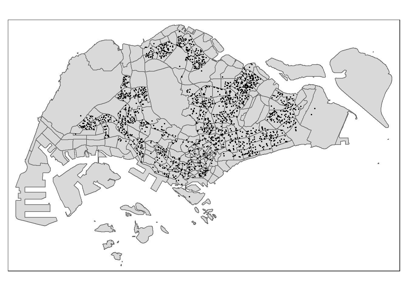
Notice that all the geospatial layers are within the same map extend. This shows that their referencing system and coordinate values are referred to similar spatial context. This is very important in any geospatial analysis.
Alternatively, we can also prepare a pin map by using the code chunk below.
Plot a map to show their spatial patterns
tmap_mode('view')tmap mode set to interactive viewingtm_shape(childcare_sf)+
tm_dots()tmap_mode('plot')tmap mode set to plottingNotice that at the interactive mode, tmap is using leaflet for R API. The advantage of this interactive pin map is it allows us to navigate and zoom around the map freely. We can also query the information of each simple feature (i.e. the point) by clicking of them. Last but not least, you can also change the background of the internet map layer. Currently, three internet map layers are provided. They are: ESRI.WorldGrayCanvas, OpenStreetMap, and ESRI.WorldTopoMap. The default is ESRI.WorldGrayCanvas.
5. Geospatial Data wrangling
Although simple feature data frame is gaining popularity again sp’s Spatial* classes, there are, however, many geospatial analysis packages require the input geospatial data in sp’s Spatial* classes. In this section, you will learn how to convert simple feature data frame to sp’s Spatial* class.
5.1 Converting sf data frames to sp’s Spatial* class
The code chunk below uses as_Spatial() of sf package to convert the three geospatial data from simple feature data frame to sp’s Spatial* class.
childcare <- as_Spatial(childcare_sf)
mpsz <- as_Spatial(mpsz_sf)
sg <- as_Spatial(sg_sf)Childcare Centres
childcareclass : SpatialPointsDataFrame
features : 1545
extent : 11203.01, 45404.24, 25667.6, 49300.88 (xmin, xmax, ymin, ymax)
crs : +proj=tmerc +lat_0=1.36666666666667 +lon_0=103.833333333333 +k=1 +x_0=28001.642 +y_0=38744.572 +ellps=WGS84 +towgs84=0,0,0,0,0,0,0 +units=m +no_defs
variables : 2
names : Name, Description
min values : kml_1, <center><table><tr><th colspan='2' align='center'><em>Attributes</em></th></tr><tr bgcolor="#E3E3F3"> <th>ADDRESSBLOCKHOUSENUMBER</th> <td></td> </tr><tr bgcolor=""> <th>ADDRESSBUILDINGNAME</th> <td></td> </tr><tr bgcolor="#E3E3F3"> <th>ADDRESSPOSTALCODE</th> <td>018989</td> </tr><tr bgcolor=""> <th>ADDRESSSTREETNAME</th> <td>1, MARINA BOULEVARD, #B1 - 01, ONE MARINA BOULEVARD, SINGAPORE 018989</td> </tr><tr bgcolor="#E3E3F3"> <th>ADDRESSTYPE</th> <td></td> </tr><tr bgcolor=""> <th>DESCRIPTION</th> <td></td> </tr><tr bgcolor="#E3E3F3"> <th>HYPERLINK</th> <td></td> </tr><tr bgcolor=""> <th>LANDXADDRESSPOINT</th> <td>0</td> </tr><tr bgcolor="#E3E3F3"> <th>LANDYADDRESSPOINT</th> <td>0</td> </tr><tr bgcolor=""> <th>NAME</th> <td>THE LITTLE SKOOL-HOUSE INTERNATIONAL PTE. LTD.</td> </tr><tr bgcolor="#E3E3F3"> <th>PHOTOURL</th> <td></td> </tr><tr bgcolor=""> <th>ADDRESSFLOORNUMBER</th> <td></td> </tr><tr bgcolor="#E3E3F3"> <th>INC_CRC</th> <td>08F73931F4A691F4</td> </tr><tr bgcolor=""> <th>FMEL_UPD_D</th> <td>20200826094036</td> </tr><tr bgcolor="#E3E3F3"> <th>ADDRESSUNITNUMBER</th> <td></td> </tr></table></center>
max values : kml_999, <center><table><tr><th colspan='2' align='center'><em>Attributes</em></th></tr><tr bgcolor="#E3E3F3"> <th>ADDRESSBLOCKHOUSENUMBER</th> <td></td> </tr><tr bgcolor=""> <th>ADDRESSBUILDINGNAME</th> <td></td> </tr><tr bgcolor="#E3E3F3"> <th>ADDRESSPOSTALCODE</th> <td>829646</td> </tr><tr bgcolor=""> <th>ADDRESSSTREETNAME</th> <td>200, PONGGOL SEVENTEENTH AVENUE, SINGAPORE 829646</td> </tr><tr bgcolor="#E3E3F3"> <th>ADDRESSTYPE</th> <td></td> </tr><tr bgcolor=""> <th>DESCRIPTION</th> <td>Child Care Services</td> </tr><tr bgcolor="#E3E3F3"> <th>HYPERLINK</th> <td></td> </tr><tr bgcolor=""> <th>LANDXADDRESSPOINT</th> <td>0</td> </tr><tr bgcolor="#E3E3F3"> <th>LANDYADDRESSPOINT</th> <td>0</td> </tr><tr bgcolor=""> <th>NAME</th> <td>RAFFLES KIDZ @ PUNGGOL PTE LTD</td> </tr><tr bgcolor="#E3E3F3"> <th>PHOTOURL</th> <td></td> </tr><tr bgcolor=""> <th>ADDRESSFLOORNUMBER</th> <td></td> </tr><tr bgcolor="#E3E3F3"> <th>INC_CRC</th> <td>379D017BF244B0FA</td> </tr><tr bgcolor=""> <th>FMEL_UPD_D</th> <td>20200826094036</td> </tr><tr bgcolor="#E3E3F3"> <th>ADDRESSUNITNUMBER</th> <td></td> </tr></table></center> URA 2014 Master Plan Planning Subzone boundary data
mpszclass : SpatialPolygonsDataFrame
features : 323
extent : 2667.538, 56396.44, 15748.72, 50256.33 (xmin, xmax, ymin, ymax)
crs : +proj=tmerc +lat_0=1.36666666666667 +lon_0=103.833333333333 +k=1 +x_0=28001.642 +y_0=38744.572 +ellps=WGS84 +towgs84=0,0,0,0,0,0,0 +units=m +no_defs
variables : 15
names : OBJECTID, SUBZONE_NO, SUBZONE_N, SUBZONE_C, CA_IND, PLN_AREA_N, PLN_AREA_C, REGION_N, REGION_C, INC_CRC, FMEL_UPD_D, X_ADDR, Y_ADDR, SHAPE_Leng, SHAPE_Area
min values : 1, 1, ADMIRALTY, AMSZ01, N, ANG MO KIO, AM, CENTRAL REGION, CR, 00F5E30B5C9B7AD8, 16409, 5092.8949, 19579.069, 871.554887798, 39437.9352703
max values : 323, 17, YUNNAN, YSSZ09, Y, YISHUN, YS, WEST REGION, WR, FFCCF172717C2EAF, 16409, 50424.7923, 49552.7904, 68083.9364708, 69748298.792 National Boundary of Singapore
sgclass : SpatialPolygonsDataFrame
features : 60
extent : 2663.926, 56047.79, 16357.98, 50244.03 (xmin, xmax, ymin, ymax)
crs : +proj=tmerc +lat_0=1.36666666666667 +lon_0=103.833333333333 +k=1 +x_0=28001.642 +y_0=38744.572 +ellps=WGS84 +towgs84=0,0,0,0,0,0,0 +units=m +no_defs
variables : 4
names : GDO_GID, MSLINK, MAPID, COSTAL_NAM
min values : 1, 1, 0, ISLAND LINK
max values : 60, 67, 0, SINGAPORE - MAIN ISLAND Notice that the geospatial data have been converted into their respective sp’s Spatial* classes now.
5.2 Converting the Spatial* class into generic sp format
spatstat requires the analytical data in ppp object form. There is no direct way to convert a Spatial* classes into ppp object. We need to convert the Spatial classes* into Spatial object first.
The codes chunk below converts the Spatial* classes into generic sp objects.
childcare_sp <- as(childcare, "SpatialPoints")
sg_sp <- as(sg, "SpatialPolygons")Next, you should display the sp objects properties as shown below.
childcare_spclass : SpatialPoints
features : 1545
extent : 11203.01, 45404.24, 25667.6, 49300.88 (xmin, xmax, ymin, ymax)
crs : +proj=tmerc +lat_0=1.36666666666667 +lon_0=103.833333333333 +k=1 +x_0=28001.642 +y_0=38744.572 +ellps=WGS84 +towgs84=0,0,0,0,0,0,0 +units=m +no_defs sg_spclass : SpatialPolygons
features : 60
extent : 2663.926, 56047.79, 16357.98, 50244.03 (xmin, xmax, ymin, ymax)
crs : +proj=tmerc +lat_0=1.36666666666667 +lon_0=103.833333333333 +k=1 +x_0=28001.642 +y_0=38744.572 +ellps=WGS84 +towgs84=0,0,0,0,0,0,0 +units=m +no_defs Do you know what are the differences between Spatial* classes and generic sp object?
Each Spatial class has a predefined structure, such as SpatialPoints, SpatialLines, SpatialPolygons, etc. This structure determines the type of geometric features represented (points, lines, polygons). Whereas,the sp object is a more generic representation of spatial data, capable of holding any type of geometric feature (points, lines, polygons). More details here.
5.3 Converting the generic sp format into spatstat’s ppp format
Now, we will use as.ppp() function of spatstat to convert the spatial data into spatstat’s ppp object format.
childcare_ppp <- as.ppp(childcare_sf)
childcare_pppMarked planar point pattern: 1545 points
marks are of storage type 'character'
window: rectangle = [11203.01, 45404.24] x [25667.6, 49300.88] unitsNow, let us plot childcare_ppp and examine the different.
plot(childcare_ppp)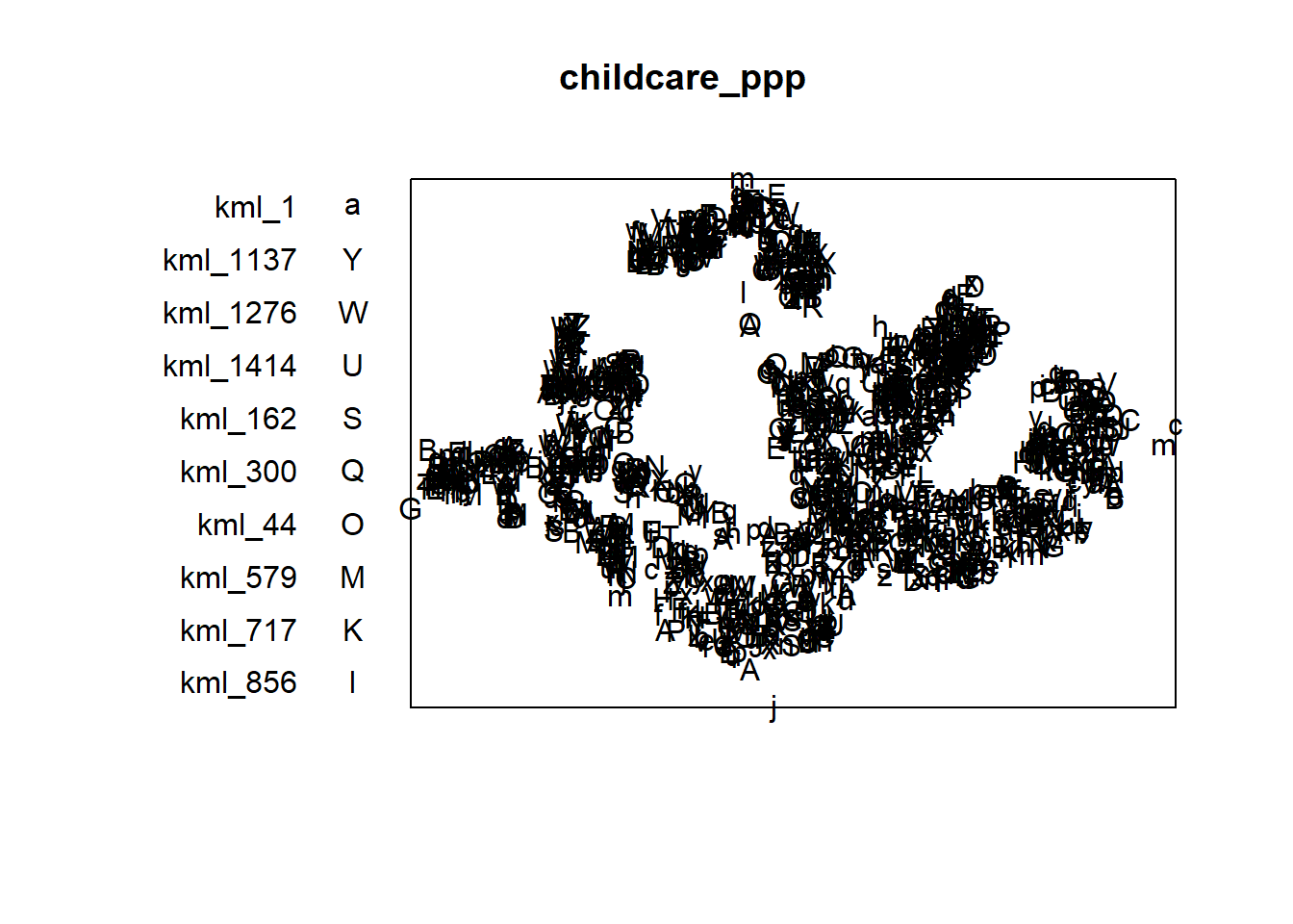
You can take a quick look at the summary statistics of the newly created ppp object by using the code chunk below.
summary(childcare_ppp)Marked planar point pattern: 1545 points
Average intensity 1.91145e-06 points per square unit
Coordinates are given to 11 decimal places
marks are of type 'character'
Summary:
Length Class Mode
1545 character character
Window: rectangle = [11203.01, 45404.24] x [25667.6, 49300.88] units
(34200 x 23630 units)
Window area = 808287000 square unitsNotice the warning message about duplicates. In spatial point patterns analysis an issue of significant is the presence of duplicates. The statistical methodology used for spatial point patterns processes is based largely on the assumption that process are simple, that is, that the points cannot be coincident.
5.4 Handling duplicated points
We can check the duplication in a ppp object by using the code chunk below.
any(duplicated(childcare_ppp))[1] FALSETo count the number of co-indicence point, we will use the multiplicity() function as shown in the code chunk below.
multiplicity(childcare_ppp) [1] 1 1 1 1 1 1 1 1 1 1 1 1 1 1 1 1 1 1 1 1 1 1 1 1 1 1 1 1 1 1 1 1 1 1 1 1 1
[38] 1 1 1 1 1 1 1 1 1 1 1 1 1 1 1 1 1 1 1 1 1 1 1 1 1 1 1 1 1 1 1 1 1 1 1 1 1
[75] 1 1 1 1 1 1 1 1 1 1 1 1 1 1 1 1 1 1 1 1 1 1 1 1 1 1 1 1 1 1 1 1 1 1 1 1 1
[112] 1 1 1 1 1 1 1 1 1 1 1 1 1 1 1 1 1 1 1 1 1 1 1 1 1 1 1 1 1 1 1 1 1 1 1 1 1
[149] 1 1 1 1 1 1 1 1 1 1 1 1 1 1 1 1 1 1 1 1 1 1 1 1 1 1 1 1 1 1 1 1 1 1 1 1 1
[186] 1 1 1 1 1 1 1 1 1 1 1 1 1 1 1 1 1 1 1 1 1 1 1 1 1 1 1 1 1 1 1 1 1 1 1 1 1
[223] 1 1 1 1 1 1 1 1 1 1 1 1 1 1 1 1 1 1 1 1 1 1 1 1 1 1 1 1 1 1 1 1 1 1 1 1 1
[260] 1 1 1 1 1 1 1 1 1 1 1 1 1 1 1 1 1 1 1 1 1 1 1 1 1 1 1 1 1 1 1 1 1 1 1 1 1
[297] 1 1 1 1 1 1 1 1 1 1 1 1 1 1 1 1 1 1 1 1 1 1 1 1 1 1 1 1 1 1 1 1 1 1 1 1 1
[334] 1 1 1 1 1 1 1 1 1 1 1 1 1 1 1 1 1 1 1 1 1 1 1 1 1 1 1 1 1 1 1 1 1 1 1 1 1
[371] 1 1 1 1 1 1 1 1 1 1 1 1 1 1 1 1 1 1 1 1 1 1 1 1 1 1 1 1 1 1 1 1 1 1 1 1 1
[408] 1 1 1 1 1 1 1 1 1 1 1 1 1 1 1 1 1 1 1 1 1 1 1 1 1 1 1 1 1 1 1 1 1 1 1 1 1
[445] 1 1 1 1 1 1 1 1 1 1 1 1 1 1 1 1 1 1 1 1 1 1 1 1 1 1 1 1 1 1 1 1 1 1 1 1 1
[482] 1 1 1 1 1 1 1 1 1 1 1 1 1 1 1 1 1 1 1 1 1 1 1 1 1 1 1 1 1 1 1 1 1 1 1 1 1
[519] 1 1 1 1 1 1 1 1 1 1 1 1 1 1 1 1 1 1 1 1 1 1 1 1 1 1 1 1 1 1 1 1 1 1 1 1 1
[556] 1 1 1 1 1 1 1 1 1 1 1 1 1 1 1 1 1 1 1 1 1 1 1 1 1 1 1 1 1 1 1 1 1 1 1 1 1
[593] 1 1 1 1 1 1 1 1 1 1 1 1 1 1 1 1 1 1 1 1 1 1 1 1 1 1 1 1 1 1 1 1 1 1 1 1 1
[630] 1 1 1 1 1 1 1 1 1 1 1 1 1 1 1 1 1 1 1 1 1 1 1 1 1 1 1 1 1 1 1 1 1 1 1 1 1
[667] 1 1 1 1 1 1 1 1 1 1 1 1 1 1 1 1 1 1 1 1 1 1 1 1 1 1 1 1 1 1 1 1 1 1 1 1 1
[704] 1 1 1 1 1 1 1 1 1 1 1 1 1 1 1 1 1 1 1 1 1 1 1 1 1 1 1 1 1 1 1 1 1 1 1 1 1
[741] 1 1 1 1 1 1 1 1 1 1 1 1 1 1 1 1 1 1 1 1 1 1 1 1 1 1 1 1 1 1 1 1 1 1 1 1 1
[778] 1 1 1 1 1 1 1 1 1 1 1 1 1 1 1 1 1 1 1 1 1 1 1 1 1 1 1 1 1 1 1 1 1 1 1 1 1
[815] 1 1 1 1 1 1 1 1 1 1 1 1 1 1 1 1 1 1 1 1 1 1 1 1 1 1 1 1 1 1 1 1 1 1 1 1 1
[852] 1 1 1 1 1 1 1 1 1 1 1 1 1 1 1 1 1 1 1 1 1 1 1 1 1 1 1 1 1 1 1 1 1 1 1 1 1
[889] 1 1 1 1 1 1 1 1 1 1 1 1 1 1 1 1 1 1 1 1 1 1 1 1 1 1 1 1 1 1 1 1 1 1 1 1 1
[926] 1 1 1 1 1 1 1 1 1 1 1 1 1 1 1 1 1 1 1 1 1 1 1 1 1 1 1 1 1 1 1 1 1 1 1 1 1
[963] 1 1 1 1 1 1 1 1 1 1 1 1 1 1 1 1 1 1 1 1 1 1 1 1 1 1 1 1 1 1 1 1 1 1 1 1 1
[1000] 1 1 1 1 1 1 1 1 1 1 1 1 1 1 1 1 1 1 1 1 1 1 1 1 1 1 1 1 1 1 1 1 1 1 1 1 1
[1037] 1 1 1 1 1 1 1 1 1 1 1 1 1 1 1 1 1 1 1 1 1 1 1 1 1 1 1 1 1 1 1 1 1 1 1 1 1
[1074] 1 1 1 1 1 1 1 1 1 1 1 1 1 1 1 1 1 1 1 1 1 1 1 1 1 1 1 1 1 1 1 1 1 1 1 1 1
[1111] 1 1 1 1 1 1 1 1 1 1 1 1 1 1 1 1 1 1 1 1 1 1 1 1 1 1 1 1 1 1 1 1 1 1 1 1 1
[1148] 1 1 1 1 1 1 1 1 1 1 1 1 1 1 1 1 1 1 1 1 1 1 1 1 1 1 1 1 1 1 1 1 1 1 1 1 1
[1185] 1 1 1 1 1 1 1 1 1 1 1 1 1 1 1 1 1 1 1 1 1 1 1 1 1 1 1 1 1 1 1 1 1 1 1 1 1
[1222] 1 1 1 1 1 1 1 1 1 1 1 1 1 1 1 1 1 1 1 1 1 1 1 1 1 1 1 1 1 1 1 1 1 1 1 1 1
[1259] 1 1 1 1 1 1 1 1 1 1 1 1 1 1 1 1 1 1 1 1 1 1 1 1 1 1 1 1 1 1 1 1 1 1 1 1 1
[1296] 1 1 1 1 1 1 1 1 1 1 1 1 1 1 1 1 1 1 1 1 1 1 1 1 1 1 1 1 1 1 1 1 1 1 1 1 1
[1333] 1 1 1 1 1 1 1 1 1 1 1 1 1 1 1 1 1 1 1 1 1 1 1 1 1 1 1 1 1 1 1 1 1 1 1 1 1
[1370] 1 1 1 1 1 1 1 1 1 1 1 1 1 1 1 1 1 1 1 1 1 1 1 1 1 1 1 1 1 1 1 1 1 1 1 1 1
[1407] 1 1 1 1 1 1 1 1 1 1 1 1 1 1 1 1 1 1 1 1 1 1 1 1 1 1 1 1 1 1 1 1 1 1 1 1 1
[1444] 1 1 1 1 1 1 1 1 1 1 1 1 1 1 1 1 1 1 1 1 1 1 1 1 1 1 1 1 1 1 1 1 1 1 1 1 1
[1481] 1 1 1 1 1 1 1 1 1 1 1 1 1 1 1 1 1 1 1 1 1 1 1 1 1 1 1 1 1 1 1 1 1 1 1 1 1
[1518] 1 1 1 1 1 1 1 1 1 1 1 1 1 1 1 1 1 1 1 1 1 1 1 1 1 1 1 1If we want to know how many locations have more than one point event, we can use the code chunk below.
sum(multiplicity(childcare_ppp) > 1)[1] 0The output shows that there are 128 duplicated point events.
To view the locations of these duplicate point events, we will plot childcare data by using the code chunk below.
tmap_mode('view')tmap mode set to interactive viewingtm_shape(childcare) +
tm_dots(alpha=0.4,
size=0.05)tmap_mode('plot')tmap mode set to plottingDo you know how to spot the duplicate points from the map shown above?
There are three ways to overcome this problem. The easiest way is to delete the duplicates. But, that will also mean that some useful point events will be lost.
The second solution is use jittering, which will add a small perturbation to the duplicate points so that they do not occupy the exact same space.
The third solution is to make each point “unique” and then attach the duplicates of the points to the patterns as marks, as attributes of the points. Then you would need analytical techniques that take into account these marks.
The code chunk below implements the jittering approach.
childcare_ppp_jit <- rjitter(childcare_ppp,
retry=TRUE,
nsim=1,
drop=TRUE)Check if any duplicated point in this geospatial data.
any(duplicated(childcare_ppp_jit))[1] FALSE5.5 Creating owin object
When analysing spatial point patterns, it is a good practice to confine the analysis with a geographical area like Singapore boundary. In spatstat, an object called owin is specially designed to represent this polygonal region.
The code chunk below is used to covert sg SpatialPolygon object into owin object of spatstat.
sg_owin <- as.owin(sg_sf)The ouput object can be displayed by using plot() function
plot(sg_owin)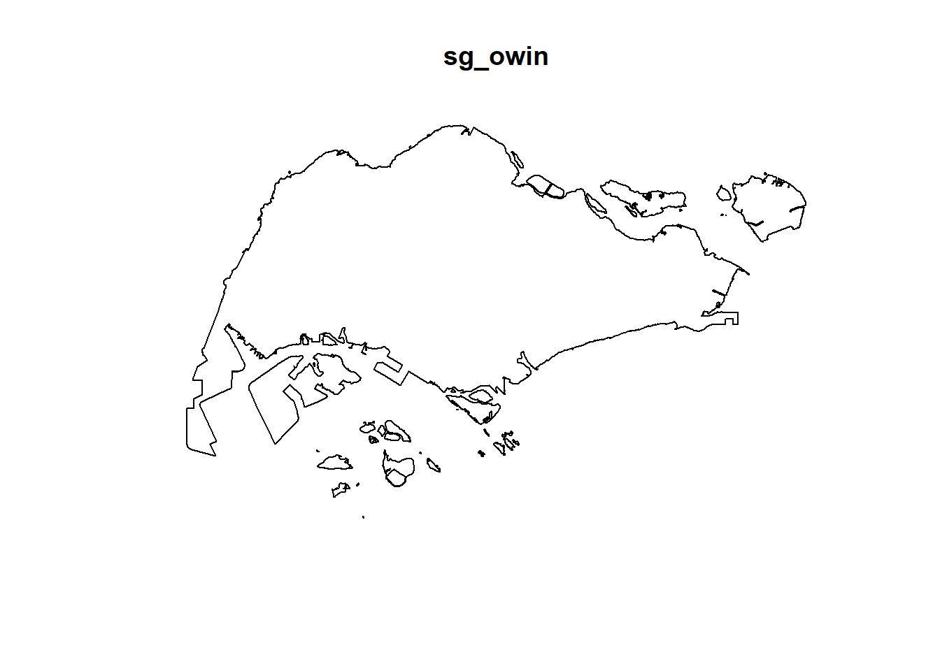
and summary() function of Base R.
summary(sg_owin)Window: polygonal boundary
50 separate polygons (1 hole)
vertices area relative.area
polygon 1 (hole) 30 -7081.18 -9.76e-06
polygon 2 55 82537.90 1.14e-04
polygon 3 90 415092.00 5.72e-04
polygon 4 49 16698.60 2.30e-05
polygon 5 38 24249.20 3.34e-05
polygon 6 976 23344700.00 3.22e-02
polygon 7 721 1927950.00 2.66e-03
polygon 8 1992 9992170.00 1.38e-02
polygon 9 330 1118960.00 1.54e-03
polygon 10 175 925904.00 1.28e-03
polygon 11 115 928394.00 1.28e-03
polygon 12 24 6352.39 8.76e-06
polygon 13 190 202489.00 2.79e-04
polygon 14 37 10170.50 1.40e-05
polygon 15 25 16622.70 2.29e-05
polygon 16 10 2145.07 2.96e-06
polygon 17 66 16184.10 2.23e-05
polygon 18 5195 636837000.00 8.78e-01
polygon 19 76 312332.00 4.31e-04
polygon 20 627 31891300.00 4.40e-02
polygon 21 20 32842.00 4.53e-05
polygon 22 42 55831.70 7.70e-05
polygon 23 67 1313540.00 1.81e-03
polygon 24 734 4690930.00 6.47e-03
polygon 25 16 3194.60 4.40e-06
polygon 26 15 4872.96 6.72e-06
polygon 27 15 4464.20 6.15e-06
polygon 28 14 5466.74 7.54e-06
polygon 29 37 5261.94 7.25e-06
polygon 30 111 662927.00 9.14e-04
polygon 31 69 56313.40 7.76e-05
polygon 32 143 145139.00 2.00e-04
polygon 33 397 2488210.00 3.43e-03
polygon 34 90 115991.00 1.60e-04
polygon 35 98 62682.90 8.64e-05
polygon 36 165 338736.00 4.67e-04
polygon 37 130 94046.50 1.30e-04
polygon 38 93 430642.00 5.94e-04
polygon 39 16 2010.46 2.77e-06
polygon 40 415 3253840.00 4.49e-03
polygon 41 30 10838.20 1.49e-05
polygon 42 53 34400.30 4.74e-05
polygon 43 26 8347.58 1.15e-05
polygon 44 74 58223.40 8.03e-05
polygon 45 327 2169210.00 2.99e-03
polygon 46 177 467446.00 6.44e-04
polygon 47 46 699702.00 9.65e-04
polygon 48 6 16841.00 2.32e-05
polygon 49 13 70087.30 9.66e-05
polygon 50 4 9459.63 1.30e-05
enclosing rectangle: [2663.93, 56047.79] x [16357.98, 50244.03] units
(53380 x 33890 units)
Window area = 725376000 square units
Fraction of frame area: 0.4015.6 Combining point events object and owin object
In this last step of geospatial data wrangling, we will extract childcare events that are located within Singapore by using the code chunk below.
childcareSG_ppp = childcare_ppp[sg_owin]The output object combined both the point and polygon feature in one ppp object class as shown below.
summary(childcareSG_ppp)Marked planar point pattern: 1545 points
Average intensity 2.129929e-06 points per square unit
Coordinates are given to 11 decimal places
marks are of type 'character'
Summary:
Length Class Mode
1545 character character
Window: polygonal boundary
50 separate polygons (1 hole)
vertices area relative.area
polygon 1 (hole) 30 -7081.18 -9.76e-06
polygon 2 55 82537.90 1.14e-04
polygon 3 90 415092.00 5.72e-04
polygon 4 49 16698.60 2.30e-05
polygon 5 38 24249.20 3.34e-05
polygon 6 976 23344700.00 3.22e-02
polygon 7 721 1927950.00 2.66e-03
polygon 8 1992 9992170.00 1.38e-02
polygon 9 330 1118960.00 1.54e-03
polygon 10 175 925904.00 1.28e-03
polygon 11 115 928394.00 1.28e-03
polygon 12 24 6352.39 8.76e-06
polygon 13 190 202489.00 2.79e-04
polygon 14 37 10170.50 1.40e-05
polygon 15 25 16622.70 2.29e-05
polygon 16 10 2145.07 2.96e-06
polygon 17 66 16184.10 2.23e-05
polygon 18 5195 636837000.00 8.78e-01
polygon 19 76 312332.00 4.31e-04
polygon 20 627 31891300.00 4.40e-02
polygon 21 20 32842.00 4.53e-05
polygon 22 42 55831.70 7.70e-05
polygon 23 67 1313540.00 1.81e-03
polygon 24 734 4690930.00 6.47e-03
polygon 25 16 3194.60 4.40e-06
polygon 26 15 4872.96 6.72e-06
polygon 27 15 4464.20 6.15e-06
polygon 28 14 5466.74 7.54e-06
polygon 29 37 5261.94 7.25e-06
polygon 30 111 662927.00 9.14e-04
polygon 31 69 56313.40 7.76e-05
polygon 32 143 145139.00 2.00e-04
polygon 33 397 2488210.00 3.43e-03
polygon 34 90 115991.00 1.60e-04
polygon 35 98 62682.90 8.64e-05
polygon 36 165 338736.00 4.67e-04
polygon 37 130 94046.50 1.30e-04
polygon 38 93 430642.00 5.94e-04
polygon 39 16 2010.46 2.77e-06
polygon 40 415 3253840.00 4.49e-03
polygon 41 30 10838.20 1.49e-05
polygon 42 53 34400.30 4.74e-05
polygon 43 26 8347.58 1.15e-05
polygon 44 74 58223.40 8.03e-05
polygon 45 327 2169210.00 2.99e-03
polygon 46 177 467446.00 6.44e-04
polygon 47 46 699702.00 9.65e-04
polygon 48 6 16841.00 2.32e-05
polygon 49 13 70087.30 9.66e-05
polygon 50 4 9459.63 1.30e-05
enclosing rectangle: [2663.93, 56047.79] x [16357.98, 50244.03] units
(53380 x 33890 units)
Window area = 725376000 square units
Fraction of frame area: 0.401Plot the newly derived childcareSG_ppp as shown below.
plot(childcareSG_ppp)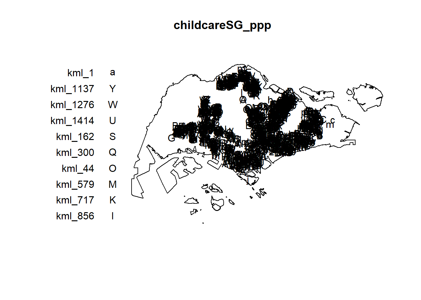
6. First-order Spatial Point Patterns Analysis
In this section, you will learn how to perform first-order SPPA by using spatstat package. The hands-on exercise will focus on:
deriving kernel density estimation (KDE) layer for visualising and exploring the intensity of point processes,
performing Confirmatory Spatial Point Patterns Analysis by using Nearest Neighbour statistics.
6.1 Kernel Density Estimation
In this section, you will learn how to compute the kernel density estimation (KDE) of childcare services in Singapore.
6.1.1 Computing kernel density estimation using automatic bandwidth selection method
The code chunk below computes a kernel density by using the following configurations of density() of spatstat:
bw.diggle() automatic bandwidth selection method. Other recommended methods are bw.CvL(), bw.scott() or bw.ppl().
The smoothing kernel used is gaussian, which is the default. Other smoothing methods are: “epanechnikov”, “quartic” or “disc”.
The intensity estimate is corrected for edge effect bias by using method described by Jones (1993) and Diggle (2010, equation 18.9). The default is FALSE.
kde_childcareSG_bw <- density(childcareSG_ppp,
sigma=bw.diggle,
edge=TRUE,
kernel="gaussian") The plot() function of Base R is then used to display the kernel density derived.
plot(kde_childcareSG_bw)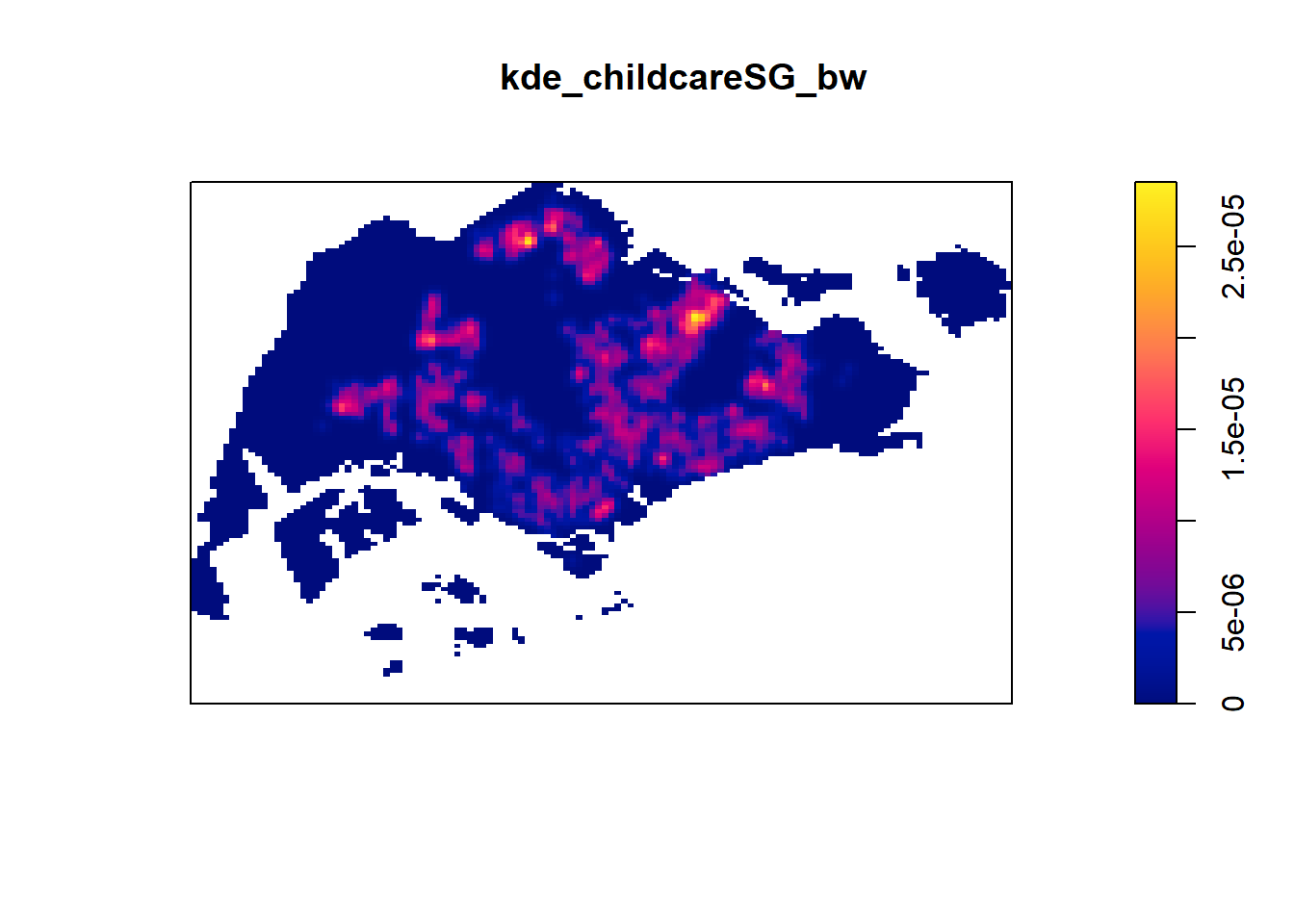
The density values of the output range from 0 to 0.000035 which is way too small to comprehend. This is because the default unit of measurement of svy21 is in meter. As a result, the density values computed is in “number of points per square meter”.
Before we move on to next section, it is good to know that you can retrieve the bandwidth used to compute the kde layer by using the code chunk below.
bw <- bw.diggle(childcareSG_ppp)
bw sigma
298.4095 6.1.2 Rescalling KDE values
In the code chunk below, rescale.ppp() is used to covert the unit of measurement from meter to kilometer.
childcareSG_ppp.km <- rescale.ppp(childcareSG_ppp, 1000, "km")Now, we can re-run density() using the resale data set and plot the output kde map.
kde_childcareSG.bw <- density(childcareSG_ppp.km, sigma=bw.diggle, edge=TRUE, kernel="gaussian")
plot(kde_childcareSG.bw)
Notice that output image looks identical to the earlier version, the only changes in the data values (refer to the legend).
6.2 Working with different automatic badwidth methods
Beside bw.diggle(), there are three other spatstat functions can be used to determine the bandwidth, they are: bw.CvL(), bw.scott(), and bw.ppl().
Let us take a look at the bandwidth return by these automatic bandwidth calculation methods by using the code chunk below.
bw.CvL(childcareSG_ppp.km) sigma
4.543278 bw.scott(childcareSG_ppp.km) sigma.x sigma.y
2.224898 1.450966 bw.ppl(childcareSG_ppp.km) sigma
0.3897114 bw.diggle(childcareSG_ppp.km) sigma
0.2984095 Baddeley et. (2016) suggested the use of the bw.ppl() algorithm because in ther experience it tends to produce the more appropriate values when the pattern consists predominantly of tight clusters. But they also insist that if the purpose of once study is to detect a single tight cluster in the midst of random noise then the bw.diggle() method seems to work best.
The code chunk beow will be used to compare the output of using bw.diggle and bw.ppl methods.
kde_childcareSG.ppl <- density(childcareSG_ppp.km,
sigma=bw.ppl,
edge=TRUE,
kernel="gaussian")
par(mfrow=c(1,2))
plot(kde_childcareSG.bw, main = "bw.diggle")
plot(kde_childcareSG.ppl, main = "bw.ppl")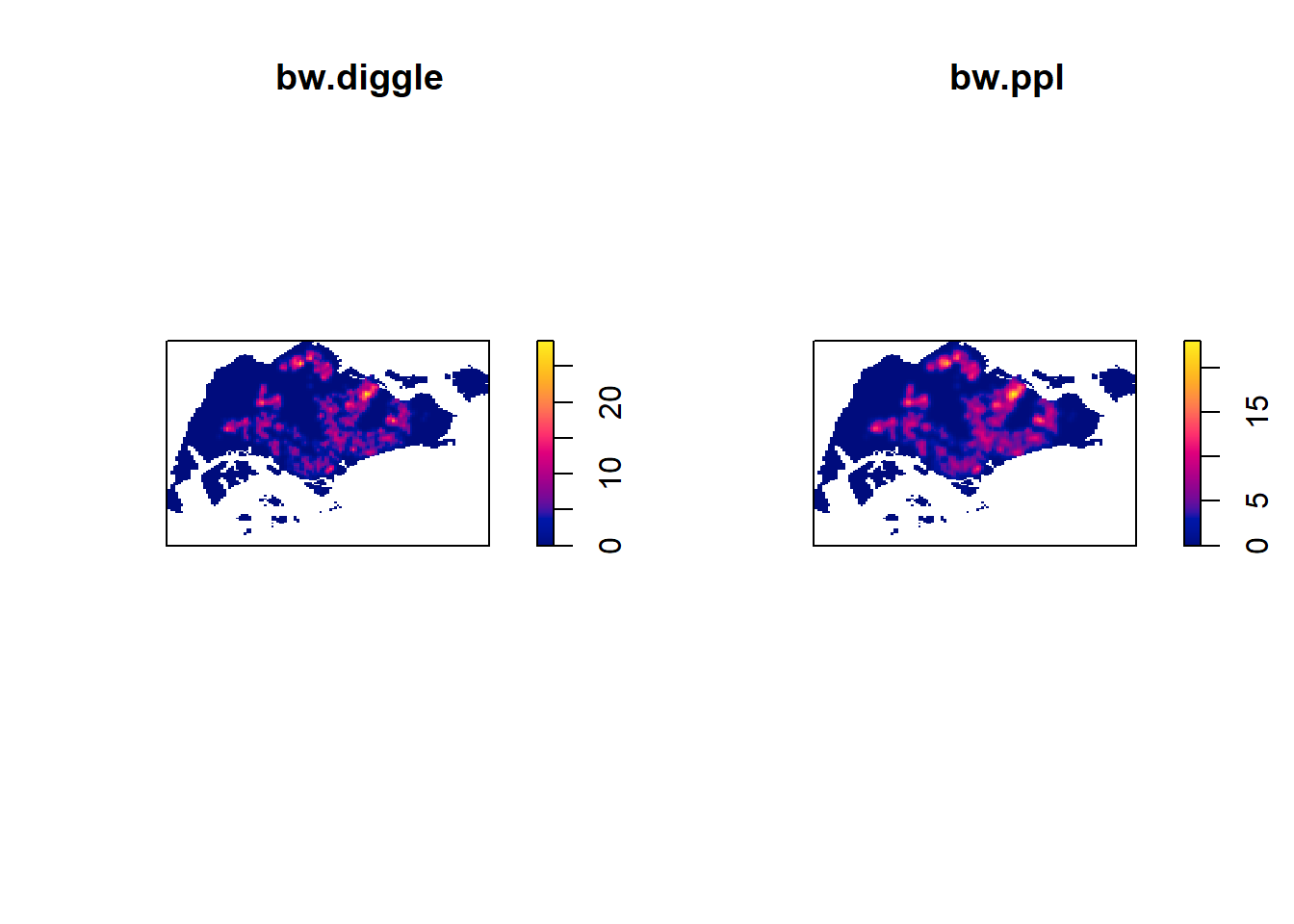
6.3 Working with different kernel methods
By default, the kernel method used in density.ppp() is gaussian. But there are three other options, namely: Epanechnikov, Quartic and Dics.
The code chunk below will be used to compute three more kernel density estimations by using these three kernel function.
par(mfrow=c(2,2))
plot(density(childcareSG_ppp.km,
sigma=bw.ppl,
edge=TRUE,
kernel="gaussian"),
main="Gaussian")
plot(density(childcareSG_ppp.km,
sigma=bw.ppl,
edge=TRUE,
kernel="epanechnikov"),
main="Epanechnikov")
plot(density(childcareSG_ppp.km,
sigma=bw.ppl,
edge=TRUE,
kernel="quartic"),
main="Quartic")
plot(density(childcareSG_ppp.km,
sigma=bw.ppl,
edge=TRUE,
kernel="disc"),
main="Disc")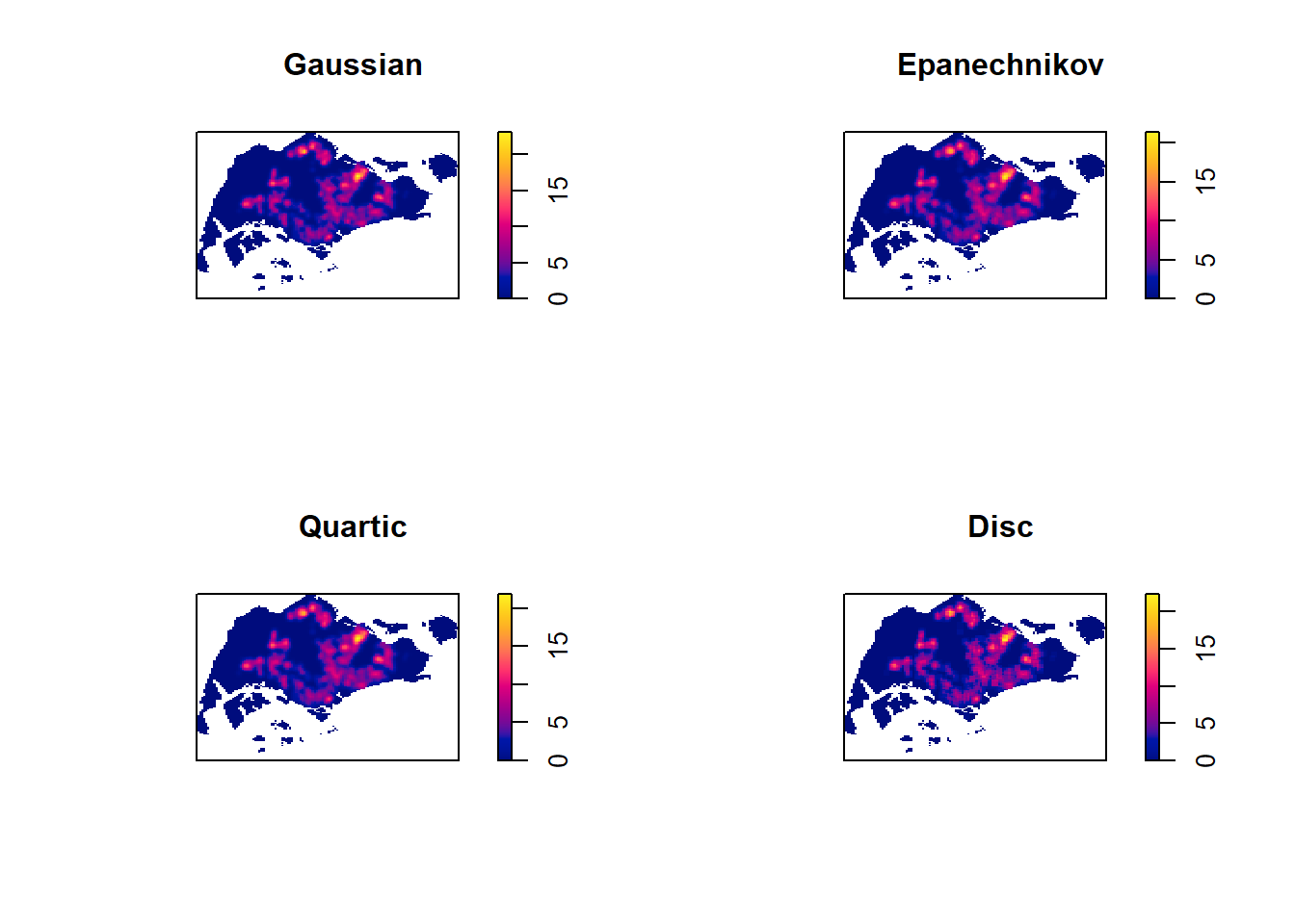
7. Fixed and Adaptive KDE
7.1 Computing KDE by using fixed bandwidth
Next, you will compute a KDE layer by defining a bandwidth of 600 meter. Notice that in the code chunk below, the sigma value used is 0.6. This is because the unit of measurement of childcareSG_ppp.km object is in kilometer, hence the 600m is 0.6km.
kde_childcareSG_600 <- density(childcareSG_ppp.km, sigma=0.6, edge=TRUE, kernel="gaussian")
plot(kde_childcareSG_600)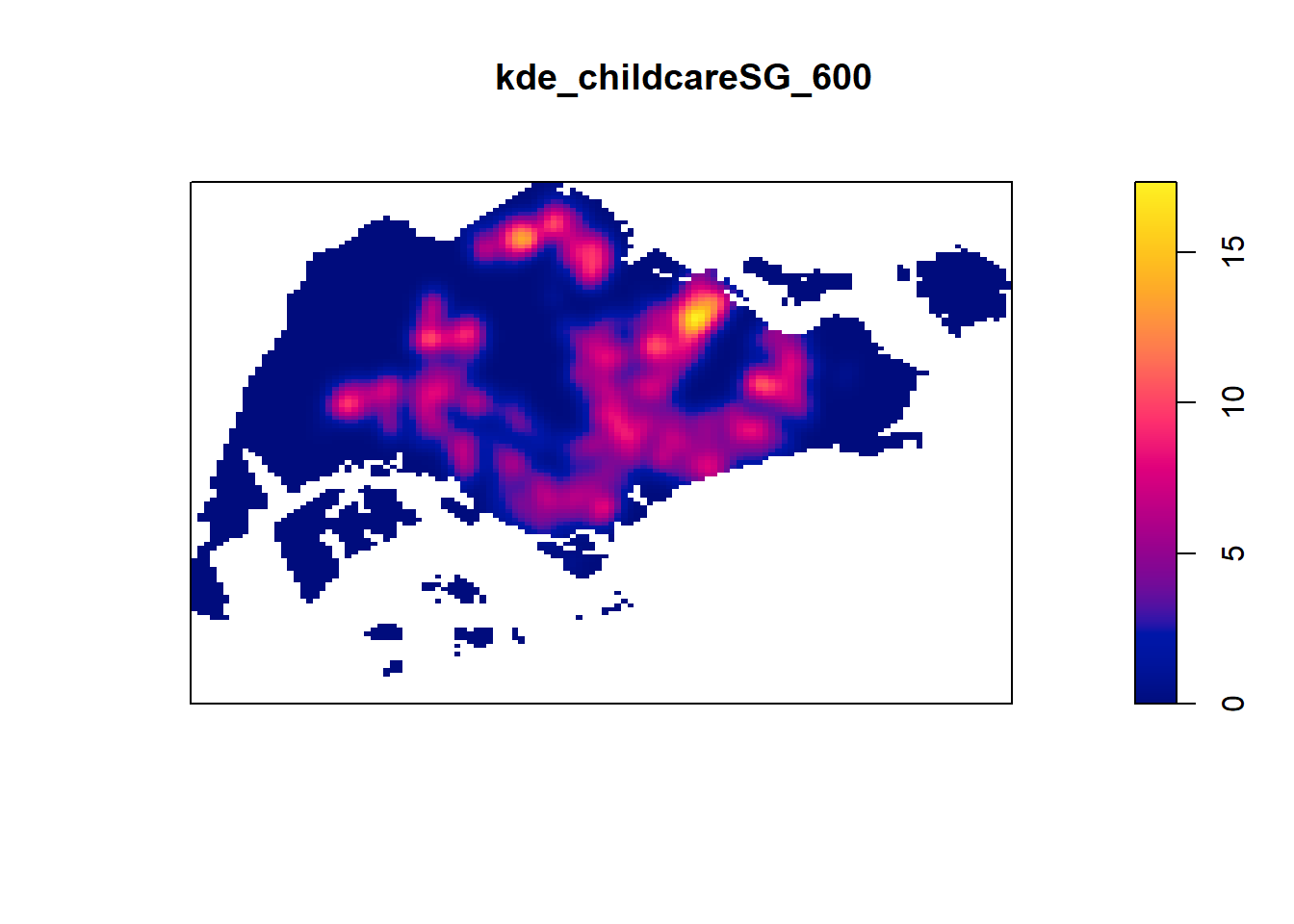
7.2 Computing KDE by using adaptive bandwidth
Fixed bandwidth method is very sensitive to highly skew distribution of spatial point patterns over geographical units for example urban versus rural. One way to overcome this problem is by using adaptive bandwidth instead.
In this section, you will learn how to derive adaptive kernel density estimation by using density.adaptive() of spatstat.
kde_childcareSG_adaptive <- adaptive.density(childcareSG_ppp.km, method="kernel")
plot(kde_childcareSG_adaptive)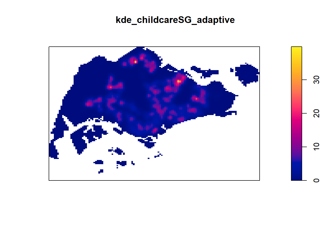
We can compare the fixed and adaptive kernel density estimation outputs by using the code chunk below.
par(mfrow=c(1,2))
plot(kde_childcareSG.bw, main = "Fixed bandwidth")
plot(kde_childcareSG_adaptive, main = "Adaptive bandwidth")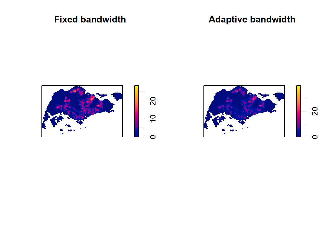
7.3 Converting KDE output into grid object.
The result is the same, we just convert it so that it is suitable for mapping purposes
# gridded_kde_childcareSG_bw <- as.SpatialGridDataFrame.im(kde_childcareSG.bw)
# spplot(gridded_kde_childcareSG_bw)The above code doesn’t work and I have changed to the below code:
raster_kde_childcareSG_bw <- raster(kde_childcareSG.bw)
gridded_kde_childcareSG_bw <- as(raster_kde_childcareSG_bw, "SpatialGridDataFrame")
spplot(gridded_kde_childcareSG_bw)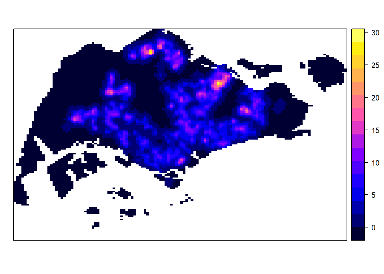
7.3.1 Converting gridded output into raster
Next, we will convert the gridded kernal density objects into RasterLayer object by using raster() of raster package.
kde_childcareSG_bw_raster <- raster(kde_childcareSG.bw)Let us take a look at the properties of kde_childcareSG_bw_raster RasterLayer.
kde_childcareSG_bw_rasterclass : RasterLayer
dimensions : 128, 128, 16384 (nrow, ncol, ncell)
resolution : 0.4170614, 0.2647348 (x, y)
extent : 2.663926, 56.04779, 16.35798, 50.24403 (xmin, xmax, ymin, ymax)
crs : NA
source : memory
names : layer
values : -8.476185e-15, 28.51831 (min, max)Notice that the crs property is NA.
7.3.2 Assigning projection systems
The code chunk below will be used to include the CRS information on kde_childcareSG_bw_raster RasterLayer.
projection(kde_childcareSG_bw_raster) <- CRS("+init=EPSG:3414")
kde_childcareSG_bw_rasterclass : RasterLayer
dimensions : 128, 128, 16384 (nrow, ncol, ncell)
resolution : 0.4170614, 0.2647348 (x, y)
extent : 2.663926, 56.04779, 16.35798, 50.24403 (xmin, xmax, ymin, ymax)
crs : +proj=tmerc +lat_0=1.36666666666667 +lon_0=103.833333333333 +k=1 +x_0=28001.642 +y_0=38744.572 +ellps=WGS84 +units=m +no_defs
source : memory
names : layer
values : -8.476185e-15, 28.51831 (min, max)Notice that the crs property is completed.
7.4 Visualising the output in tmap
Finally, we will display the raster in cartographic quality map using tmap package.
tm_shape(kde_childcareSG_bw_raster) +
tm_raster("layer", palette = "viridis") +
tm_layout(legend.position = c("right", "bottom"), frame = FALSE)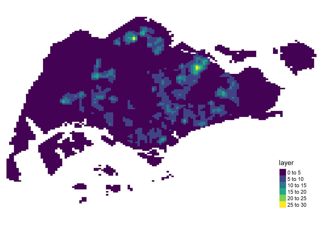
Notice that the raster values are encoded explicitly onto the raster pixel using the values in “v”” field.
7.5 Comparing Spatial Point Patterns using KDE
In this section, you will learn how to compare KDE of childcare at Punggol, Tampines, Chua Chu Kang and Jurong West planning areas.
7.5.1 Extracting study area
The code chunk below will be used to extract the target planning areas.
pg <- mpsz_sf %>%
filter(PLN_AREA_N == "PUNGGOL")
tm <- mpsz_sf %>%
filter(PLN_AREA_N == "TAMPINES")
ck <- mpsz_sf %>%
filter(PLN_AREA_N == "CHOA CHU KANG")
jw <- mpsz_sf %>%
filter(PLN_AREA_N == "JURONG WEST")Plotting target planning areas
par(mfrow=c(2,2))
plot(pg, main = "Punggol")Warning: plotting the first 9 out of 15 attributes; use max.plot = 15 to plot
all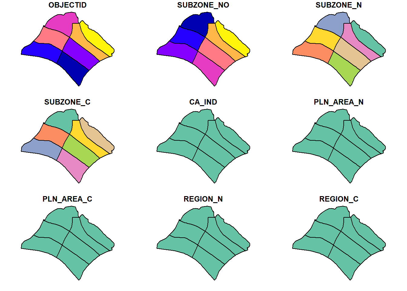
plot(tm, main = "Tampines")Warning: plotting the first 9 out of 15 attributes; use max.plot = 15 to plot
all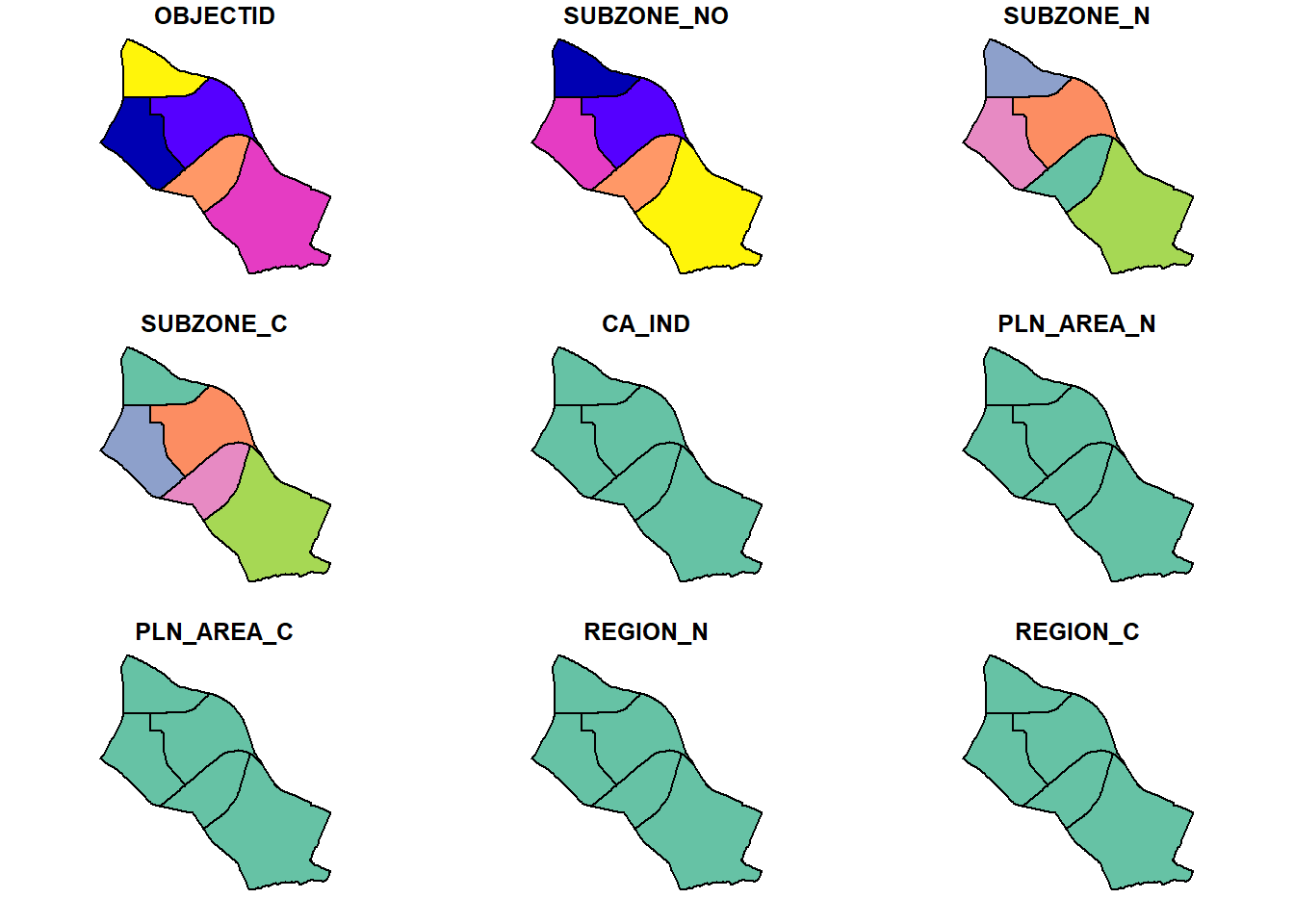
plot(ck, main = "Choa Chu Kang")Warning: plotting the first 10 out of 15 attributes; use max.plot = 15 to plot
all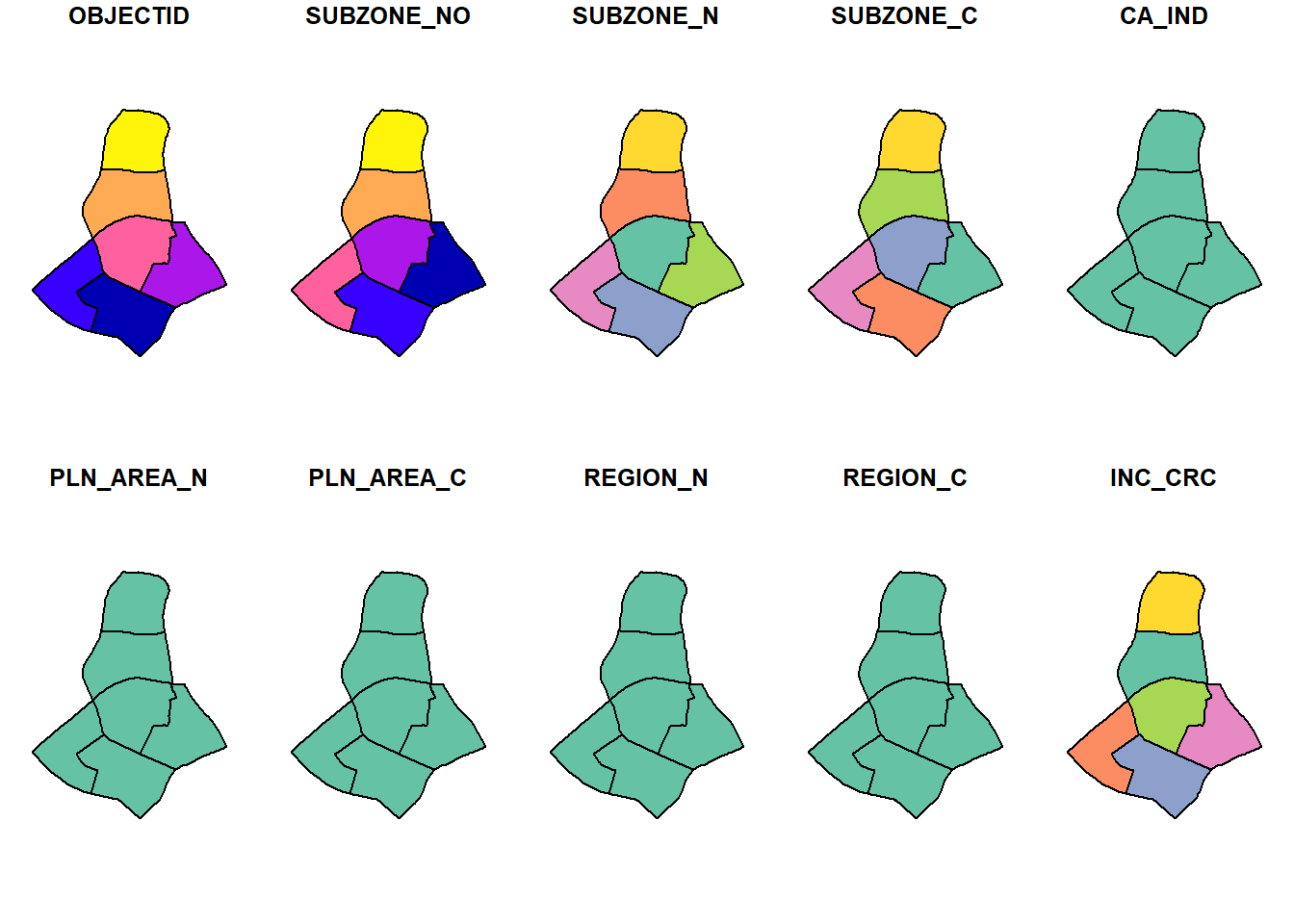
plot(jw, main = "Jurong West")Warning: plotting the first 9 out of 15 attributes; use max.plot = 15 to plot
all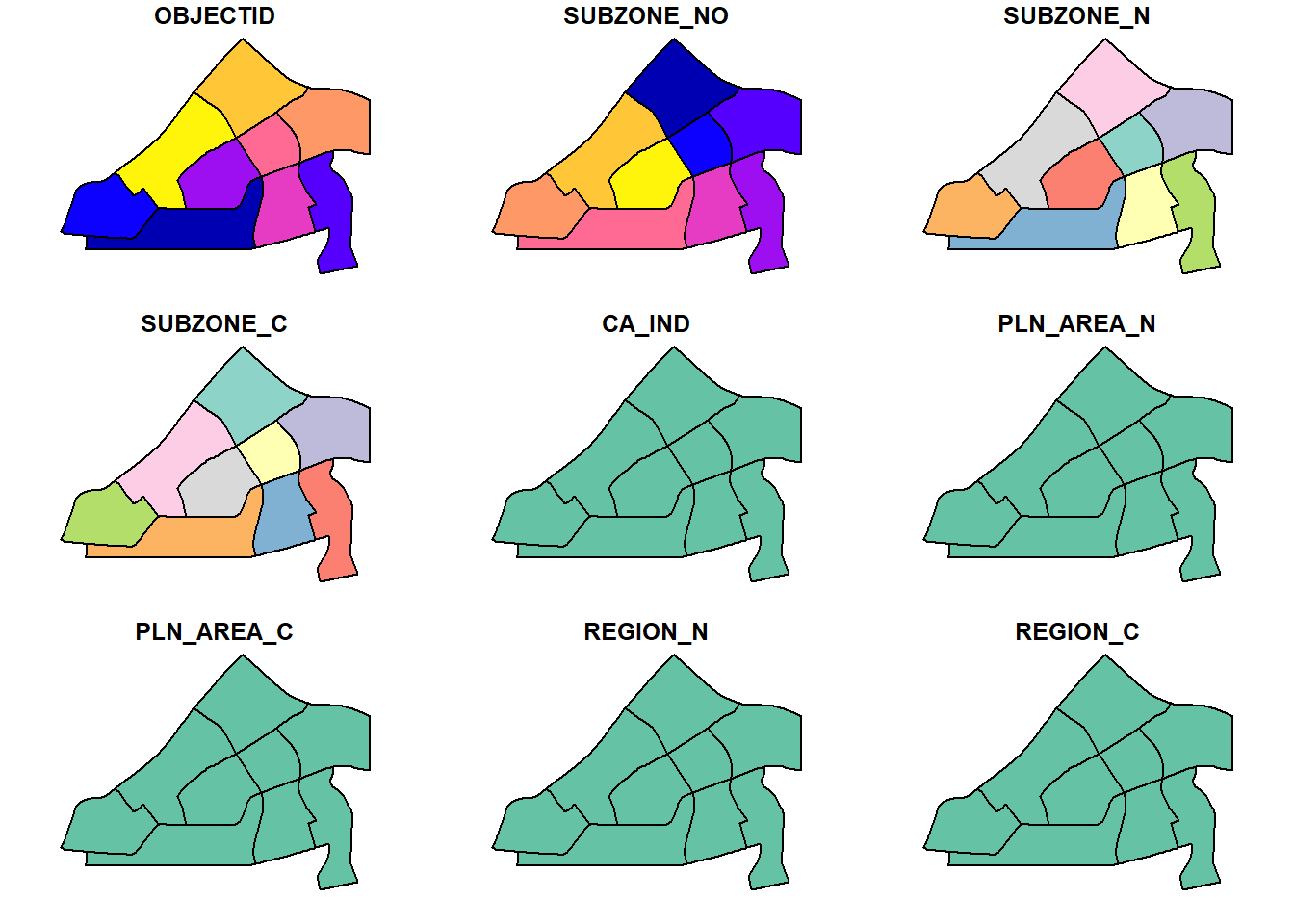
7.5.2 Creating owin object
Now, we will convert these sf objects into owin objects that is required by spatstat.
pg_owin = as.owin(pg)
tm_owin = as.owin(tm)
ck_owin = as.owin(ck)
jw_owin = as.owin(jw)7.5.3 Combining childcare points and the study area
By using the code chunk below, we are able to extract childcare that is within the specific region to do our analysis later on.
childcare_pg_ppp = childcare_ppp_jit[pg_owin]
childcare_tm_ppp = childcare_ppp_jit[tm_owin]
childcare_ck_ppp = childcare_ppp_jit[ck_owin]
childcare_jw_ppp = childcare_ppp_jit[jw_owin]Next, rescale.ppp() function is used to trasnform the unit of measurement from metre to kilometre.
childcare_pg_ppp.km = rescale.ppp(childcare_pg_ppp, 1000, "km")
childcare_tm_ppp.km = rescale.ppp(childcare_tm_ppp, 1000, "km")
childcare_ck_ppp.km = rescale.ppp(childcare_ck_ppp, 1000, "km")
childcare_jw_ppp.km = rescale.ppp(childcare_jw_ppp, 1000, "km")The code chunk below is used to plot these four study areas and the locations of the childcare centres.
par(mfrow=c(2,2))
plot(childcare_pg_ppp.km, main="Punggol")
plot(childcare_tm_ppp.km, main="Tampines")
plot(childcare_ck_ppp.km, main="Choa Chu Kang")
plot(childcare_jw_ppp.km, main="Jurong West")
7.5.4 Computing KDE
The code chunk below will be used to compute the KDE of these four planning area. bw.diggle method is used to derive the bandwidth of each
par(mfrow=c(2,2))
plot(density(childcare_pg_ppp.km,
sigma=bw.diggle,
edge=TRUE,
kernel="gaussian"),
main="Punggol")
plot(density(childcare_tm_ppp.km,
sigma=bw.diggle,
edge=TRUE,
kernel="gaussian"),
main="Tampines")
plot(density(childcare_ck_ppp.km,
sigma=bw.diggle,
edge=TRUE,
kernel="gaussian"),
main="Choa Chu Kang")
plot(density(childcare_jw_ppp.km,
sigma=bw.diggle,
edge=TRUE,
kernel="gaussian"),
main="Jurong West")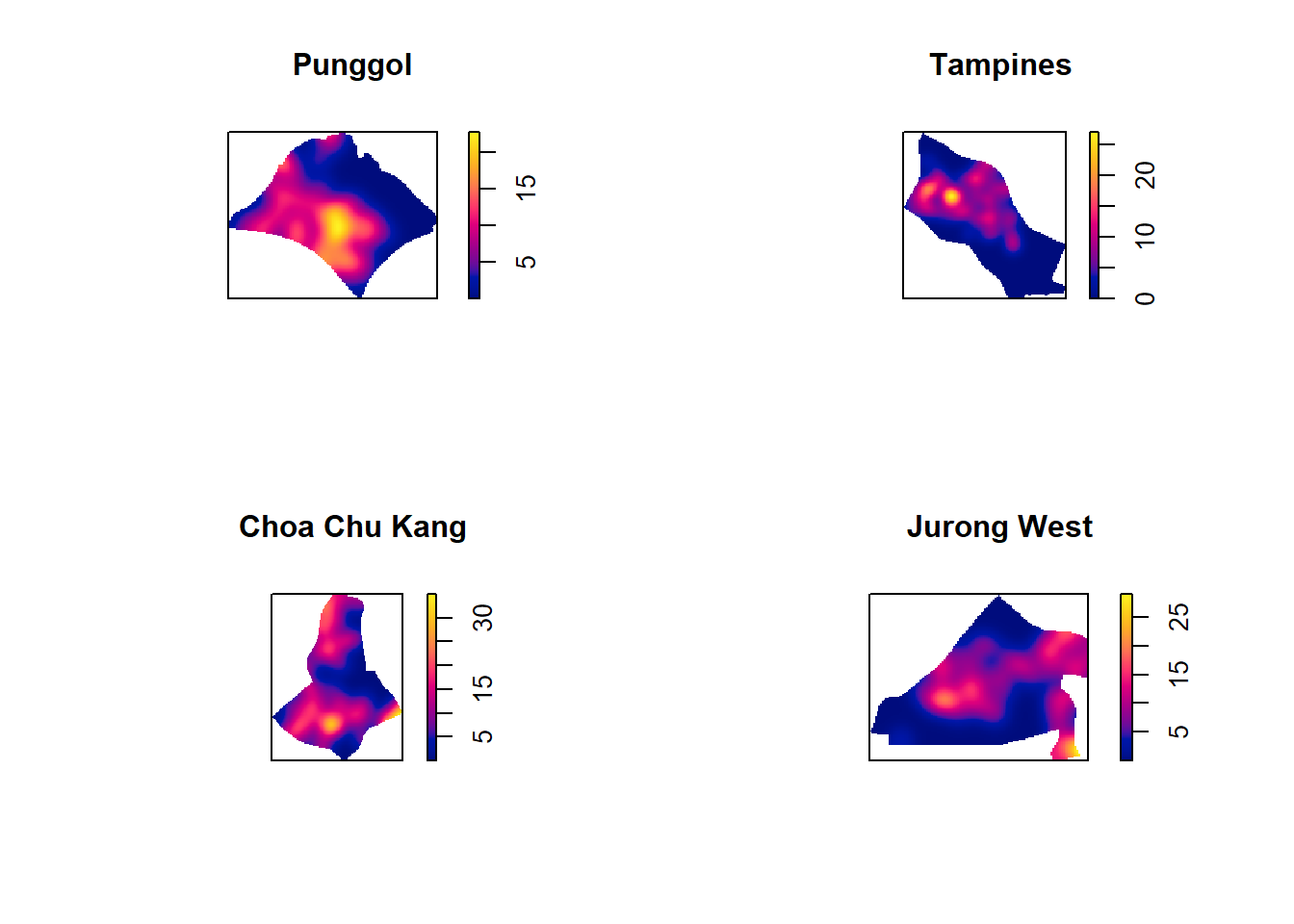
7.5.5 Computing fixed bandwidth KDE
For comparison purposes, we will use 250m as the bandwidth.
par(mfrow=c(2,2))
plot(density(childcare_ck_ppp.km,
sigma=0.25,
edge=TRUE,
kernel="gaussian"),
main="Chou Chu Kang")
plot(density(childcare_jw_ppp.km,
sigma=0.25,
edge=TRUE,
kernel="gaussian"),
main="Jurong West")
plot(density(childcare_pg_ppp.km,
sigma=0.25,
edge=TRUE,
kernel="gaussian"),
main="Punggol")
plot(density(childcare_tm_ppp.km,
sigma=0.25,
edge=TRUE,
kernel="gaussian"),
main="Tampines")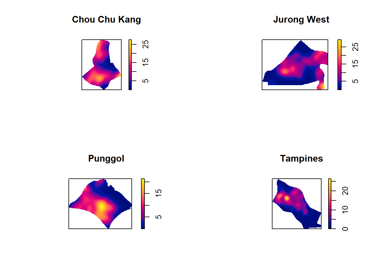
8. Nearest Neighbour Analysis
In this section, we will perform the Clark-Evans test of aggregation for a spatial point pattern by using clarkevans.test() of statspat.
The test hypotheses are:
Ho = The distribution of childcare services are randomly distributed.
H1= The distribution of childcare services are not randomly distributed.
The 95% confident interval will be used.
8.1 Testing spatial point patterns using Clark and Evans Test
clarkevans.test(childcareSG_ppp,
correction="none",
clipregion="sg_owin",
alternative=c("clustered"),
nsim=99)
Clark-Evans test
No edge correction
Z-test
data: childcareSG_ppp
R = 0.55631, p-value < 2.2e-16
alternative hypothesis: clustered (R < 1)What conclusion can you draw from the test result?
The test result indicates a significant clustering of childcare centers in Singapore.
R value: 0.55631 This value is significantly different from 0, suggesting a deviation from randomness. A higher R value indicates a stronger degree of clustering.
p-value: < 2.2e-16 This extremely small p-value provides strong evidence against the null hypothesis of complete randomness. It indicates that the observed clustering is highly unlikely to be due to chance.
Based on the test results, it can be concluded that the distribution of childcare centers in Singapore exhibits a significant degree of clustering. This suggests that there are factors influencing the location of childcare centers, such as population density, accessibility, or existing infrastructure.
8.2 Clark and Evans Test: Choa Chu Kang planning area
In the code chunk below, clarkevans.test() of spatstat is used to performs Clark-Evans test of aggregation for childcare centre in Choa Chu Kang planning area.
clarkevans.test(childcare_ck_ppp,
correction="none",
clipregion=NULL,
alternative=c("two.sided"),
nsim=999)
Clark-Evans test
No edge correction
Z-test
data: childcare_ck_ppp
R = 0.93251, p-value = 0.3133
alternative hypothesis: two-sided8.3 Clark and Evans Test: Tampines planning area
In the code chunk below, the similar test is used to analyse the spatial point patterns of childcare centre in Tampines planning area.
clarkevans.test(childcare_tm_ppp,
correction="none",
clipregion=NULL,
alternative=c("two.sided"),
nsim=999)
Clark-Evans test
No edge correction
Z-test
data: childcare_tm_ppp
R = 0.7795, p-value = 6.905e-05
alternative hypothesis: two-sided