install.packages("maptools",
repos = "https://packagemanager.posit.co/cran/2023-10-13")In-class Exercise 2
Issue 1: Installing maptools
maptools is retired and binary is removed from CRAN. However, I can download from Posit Public Package Manager snapshots by using the code chunk below.
After the installation is completed, it is important to edit the code chunk as shown below in order to avoid maptools being download and install repetitively every time the Quarto document been rendered.
Issue 2: Creating coastal outline
In sf package, there are two functions allow us to combine multiple simple features into one simple features. They are st_combine() and st_union().
st_combine()returns a single, combined geometry, with no resolved boundaries; returned geometries may well be invalid.If y is missing,
st_union(x)returns a single geometry with resolved boundaries, else the geometries for all unioned pairs of x[i] and y[j].
pacman::p_load(sf, raster, spatstat, tmap, tidyverse)childcare_sf <- st_read("data/child-care-services-geojson.geojson") %>%
st_transform(crs = 3414)Reading layer `child-care-services-geojson' from data source
`C:\Users\user\OneDrive - Singapore Management University\MITB\6. Geospatial Analytics and Applications\jeffleesl\ISSS626-GAA\In-class_Ex\In-class_Ex02\data\child-care-services-geojson.geojson'
using driver `GeoJSON'
Simple feature collection with 1545 features and 2 fields
Geometry type: POINT
Dimension: XYZ
Bounding box: xmin: 103.6824 ymin: 1.248403 xmax: 103.9897 ymax: 1.462134
z_range: zmin: 0 zmax: 0
Geodetic CRS: WGS 84mpsz_sf <- st_read(dsn = "data",
layer = "MP14_SUBZONE_WEB_PL") %>%
st_transform(crs = 3414)Reading layer `MP14_SUBZONE_WEB_PL' from data source
`C:\Users\user\OneDrive - Singapore Management University\MITB\6. Geospatial Analytics and Applications\jeffleesl\ISSS626-GAA\In-class_Ex\In-class_Ex02\data'
using driver `ESRI Shapefile'
Simple feature collection with 323 features and 15 fields
Geometry type: MULTIPOLYGON
Dimension: XY
Bounding box: xmin: 2667.538 ymin: 15748.72 xmax: 56396.44 ymax: 50256.33
Projected CRS: SVY21sg_sf <- st_read(dsn = "data",
layer="CostalOutline") %>%
st_transform(crs = 3414)Reading layer `CostalOutline' from data source
`C:\Users\user\OneDrive - Singapore Management University\MITB\6. Geospatial Analytics and Applications\jeffleesl\ISSS626-GAA\In-class_Ex\In-class_Ex02\data'
using driver `ESRI Shapefile'
Simple feature collection with 60 features and 4 fields
Geometry type: POLYGON
Dimension: XY
Bounding box: xmin: 2663.926 ymin: 16357.98 xmax: 56047.79 ymax: 50244.03
Projected CRS: SVY21Working with st_union()
The code chunk below, st_union()is used to derive the coastal outline sf tibble data.frame.
sg_sf <- mpsz_sf %>%
  st_union()
plot(sg_sf) 
sg_sf will look similar to the figure below.
plot(sg_sf) 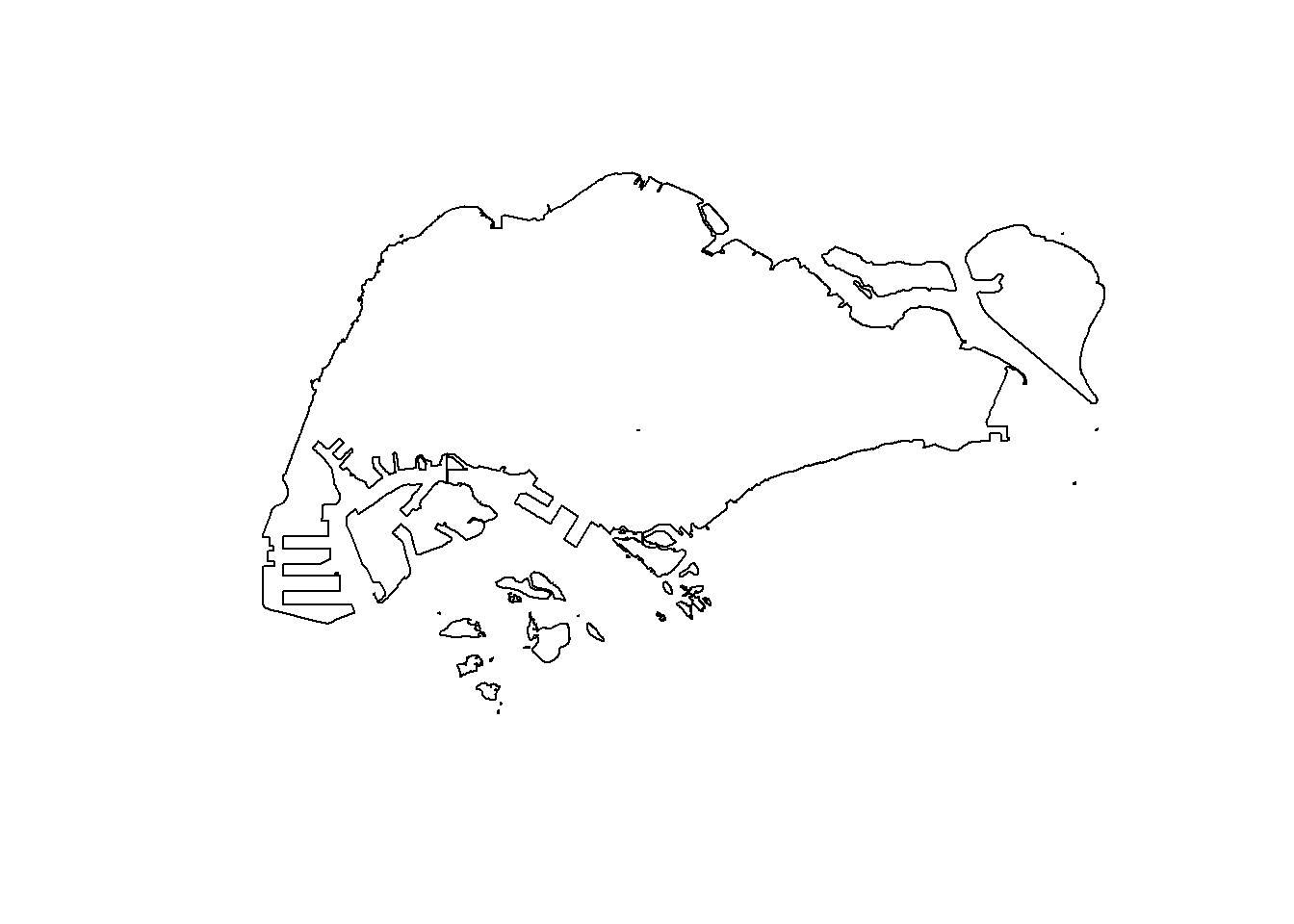
Introducing spatstat package
spatstat R package is a comprehensive open-source toolbox for analysing Spatial Point Patterns. Focused mainly on two-dimensional point patterns, including multitype or marked points, in any spatial region.
Spatstat
spatstat sub-packages
The spatstat package now contains only documentation and introductory material. It provides beginner’s introductions, vignettes, interactive demonstration scripts, and a few help files summarising the package.
The spatstat.data package now contains all the datasets for spatstat.
The spatstat.utils package contains basic utility functions for spatstat.
The spatstat.univar package contains functions for estimating and manipulating probability distributions of one-dimensional random variables.
The spatstat.sparse package contains functions for manipulating sparse arrays and performing linear algebra.
The spatstat.geom package contains definitions of spatial objects (such as point patterns, windows and pixel images) and code which performs geometrical operations.
The spatstat.random package contains functions for random generation of spatial patterns and random simulation of models.
The spatstat.explore package contains the code for exploratory data analysis and nonparametric analysis of spatial data.
The spatstat.model package contains the code for model-fitting, model diagnostics, and formal inference.
The spatstat.linnet package defines spatial data on a linear network, and performs geometrical operations and statistical analysis on such data.
Creating ppp objects from sf data.frame
Instead of using the two steps approaches discussed in Hands-on Exercise 3 to create the ppp objects, in this section you will learn how to work with sf data.frame.
In the code chunk below, as.ppp() of spatstat.geom package is used to derive an ppp object layer directly from a sf tibble data.frame.
childcare_ppp <- as.ppp(childcare_sf)Warning in as.ppp.sf(childcare_sf): only first attribute column is used for
marksplot(childcare_ppp)Warning in default.charmap(ntypes, chars): Too many types to display every type
as a different characterWarning: Only 10 out of 1545 symbols are shown in the symbol map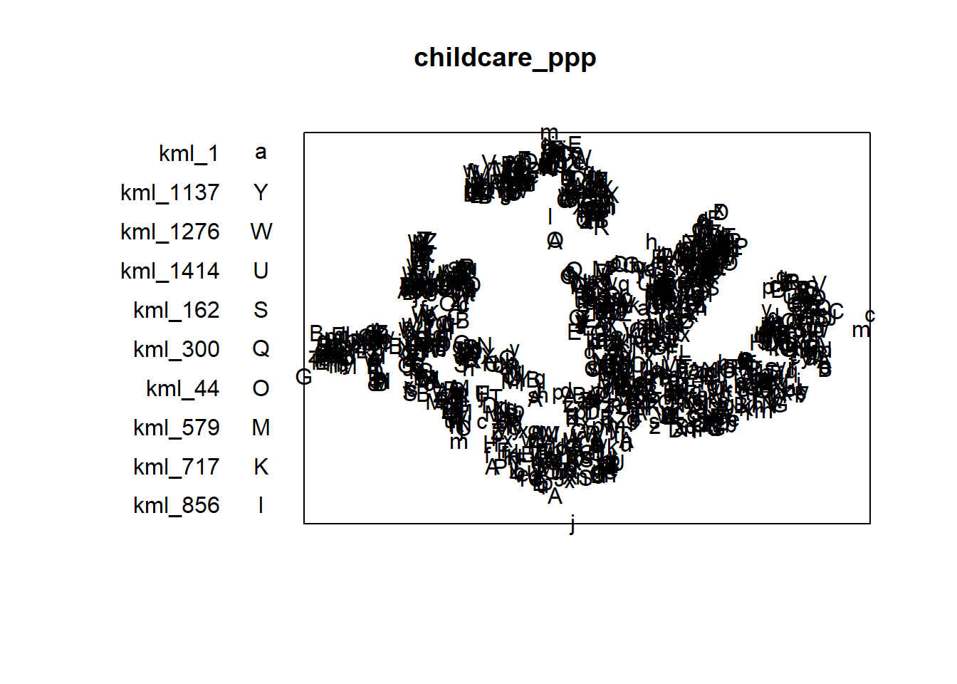
Next, summary() can be used to reveal the properties of the newly created ppp objects.
summary(childcare_ppp)Marked planar point pattern: 1545 points
Average intensity 1.91145e-06 points per square unit
Coordinates are given to 11 decimal places
marks are of type 'character'
Summary:
Length Class Mode
1545 character character
Window: rectangle = [11203.01, 45404.24] x [25667.6, 49300.88] units
(34200 x 23630 units)
Window area = 808287000 square unitsCreating owin object from sf data.frame
In the code chunk as.owin() of spatstat.geom is used to create an owin object class from polygon sf tibble data.frame.
sg_owin <- as.owin(sg_sf)
plot(sg_owin)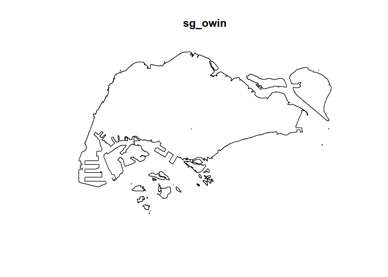
Next, summary() function is used to display the summary information of the owin object class.
summary(sg_owin)Window: polygonal boundary
80 separate polygons (35 holes)
vertices area relative.area
polygon 1 14650 6.97996e+08 8.93e-01
polygon 2 (hole) 3 -2.21090e+00 -2.83e-09
polygon 3 285 1.61128e+06 2.06e-03
polygon 4 (hole) 3 -2.05920e-03 -2.63e-12
polygon 5 (hole) 3 -8.83647e-03 -1.13e-11
polygon 6 668 5.40368e+07 6.91e-02
polygon 7 44 2.26577e+03 2.90e-06
polygon 8 27 1.50315e+04 1.92e-05
polygon 9 711 1.28815e+07 1.65e-02
polygon 10 (hole) 36 -4.01660e+04 -5.14e-05
polygon 11 (hole) 317 -5.11280e+04 -6.54e-05
polygon 12 (hole) 3 -3.41405e-01 -4.37e-10
polygon 13 (hole) 3 -2.89050e-05 -3.70e-14
polygon 14 77 3.29939e+05 4.22e-04
polygon 15 30 2.80002e+04 3.58e-05
polygon 16 (hole) 3 -2.83151e-01 -3.62e-10
polygon 17 71 8.18750e+03 1.05e-05
polygon 18 (hole) 3 -1.68316e-04 -2.15e-13
polygon 19 (hole) 36 -7.79904e+03 -9.97e-06
polygon 20 (hole) 4 -2.05611e-02 -2.63e-11
polygon 21 (hole) 3 -2.18000e-06 -2.79e-15
polygon 22 (hole) 3 -3.65501e-03 -4.67e-12
polygon 23 (hole) 3 -4.95057e-02 -6.33e-11
polygon 24 (hole) 3 -3.99521e-02 -5.11e-11
polygon 25 (hole) 3 -6.62377e-01 -8.47e-10
polygon 26 (hole) 3 -2.09065e-03 -2.67e-12
polygon 27 91 1.49663e+04 1.91e-05
polygon 28 (hole) 26 -1.25665e+03 -1.61e-06
polygon 29 (hole) 349 -1.21433e+03 -1.55e-06
polygon 30 (hole) 20 -4.39069e+00 -5.62e-09
polygon 31 (hole) 48 -1.38338e+02 -1.77e-07
polygon 32 (hole) 28 -1.99862e+01 -2.56e-08
polygon 33 40 1.38607e+04 1.77e-05
polygon 34 (hole) 40 -6.00381e+03 -7.68e-06
polygon 35 (hole) 7 -1.40545e-01 -1.80e-10
polygon 36 (hole) 12 -8.36709e+01 -1.07e-07
polygon 37 45 2.51218e+03 3.21e-06
polygon 38 142 3.22293e+03 4.12e-06
polygon 39 148 3.10395e+03 3.97e-06
polygon 40 75 1.73526e+04 2.22e-05
polygon 41 83 5.28920e+03 6.76e-06
polygon 42 211 4.70521e+05 6.02e-04
polygon 43 106 3.04104e+03 3.89e-06
polygon 44 266 1.50631e+06 1.93e-03
polygon 45 71 5.63061e+03 7.20e-06
polygon 46 10 1.99717e+02 2.55e-07
polygon 47 478 2.06120e+06 2.64e-03
polygon 48 155 2.67502e+05 3.42e-04
polygon 49 1027 1.27782e+06 1.63e-03
polygon 50 (hole) 3 -1.16959e-03 -1.50e-12
polygon 51 65 8.42861e+04 1.08e-04
polygon 52 47 3.82087e+04 4.89e-05
polygon 53 6 4.50259e+02 5.76e-07
polygon 54 132 9.53357e+04 1.22e-04
polygon 55 (hole) 3 -3.23310e-04 -4.13e-13
polygon 56 4 2.69313e+02 3.44e-07
polygon 57 (hole) 3 -1.46474e-03 -1.87e-12
polygon 58 1045 4.44510e+06 5.68e-03
polygon 59 22 6.74651e+03 8.63e-06
polygon 60 64 3.43149e+04 4.39e-05
polygon 61 (hole) 3 -1.98390e-03 -2.54e-12
polygon 62 (hole) 4 -1.13774e-02 -1.46e-11
polygon 63 14 5.86546e+03 7.50e-06
polygon 64 95 5.96187e+04 7.62e-05
polygon 65 (hole) 4 -1.86410e-02 -2.38e-11
polygon 66 (hole) 3 -5.12482e-03 -6.55e-12
polygon 67 (hole) 3 -1.96410e-03 -2.51e-12
polygon 68 (hole) 3 -5.55856e-03 -7.11e-12
polygon 69 234 2.08755e+06 2.67e-03
polygon 70 10 4.90942e+02 6.28e-07
polygon 71 234 4.72886e+05 6.05e-04
polygon 72 (hole) 13 -3.91907e+02 -5.01e-07
polygon 73 15 4.03300e+04 5.16e-05
polygon 74 227 1.10308e+06 1.41e-03
polygon 75 10 6.60195e+03 8.44e-06
polygon 76 19 3.09221e+04 3.95e-05
polygon 77 145 9.61782e+05 1.23e-03
polygon 78 30 4.28933e+03 5.49e-06
polygon 79 37 1.29481e+04 1.66e-05
polygon 80 4 9.47108e+01 1.21e-07
enclosing rectangle: [2667.54, 56396.44] x [15748.72, 50256.33] units
(53730 x 34510 units)
Window area = 781945000 square units
Fraction of frame area: 0.422Combining point events object and owin object
In the code chunk as.owin() of spatstat.geom is used to create an owin object class from polygon sf tibble data.frame.
Using the step you learned from Hands-on Exercise 3, create an ppp object by combining childcare_ppp and sg_owin.
Next, summary() function is used to display the summary information of the owin object class.
childcareSG_ppp = childcare_ppp[sg_owin]The output object combined both the point and polygon feature in one ppp object class as shown below.
plot(childcareSG_ppp)Warning in default.charmap(ntypes, chars): Too many types to display every type
as a different characterWarning: Only 10 out of 1545 symbols are shown in the symbol map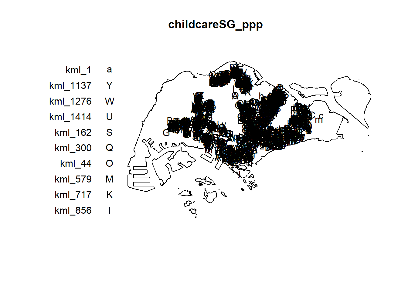
Kernel Density Estimation of Spatial Point Event
The code chunk below re-scale the unit of measurement from metre to kilometre before performing KDE.
childcareSG_ppp.km <- rescale.ppp(childcareSG_ppp,
                                  1000,
                                  "km")

kde_childcareSG_adaptive <- adaptive.density(
  childcareSG_ppp.km,
  method="kernel")
plot(kde_childcareSG_adaptive)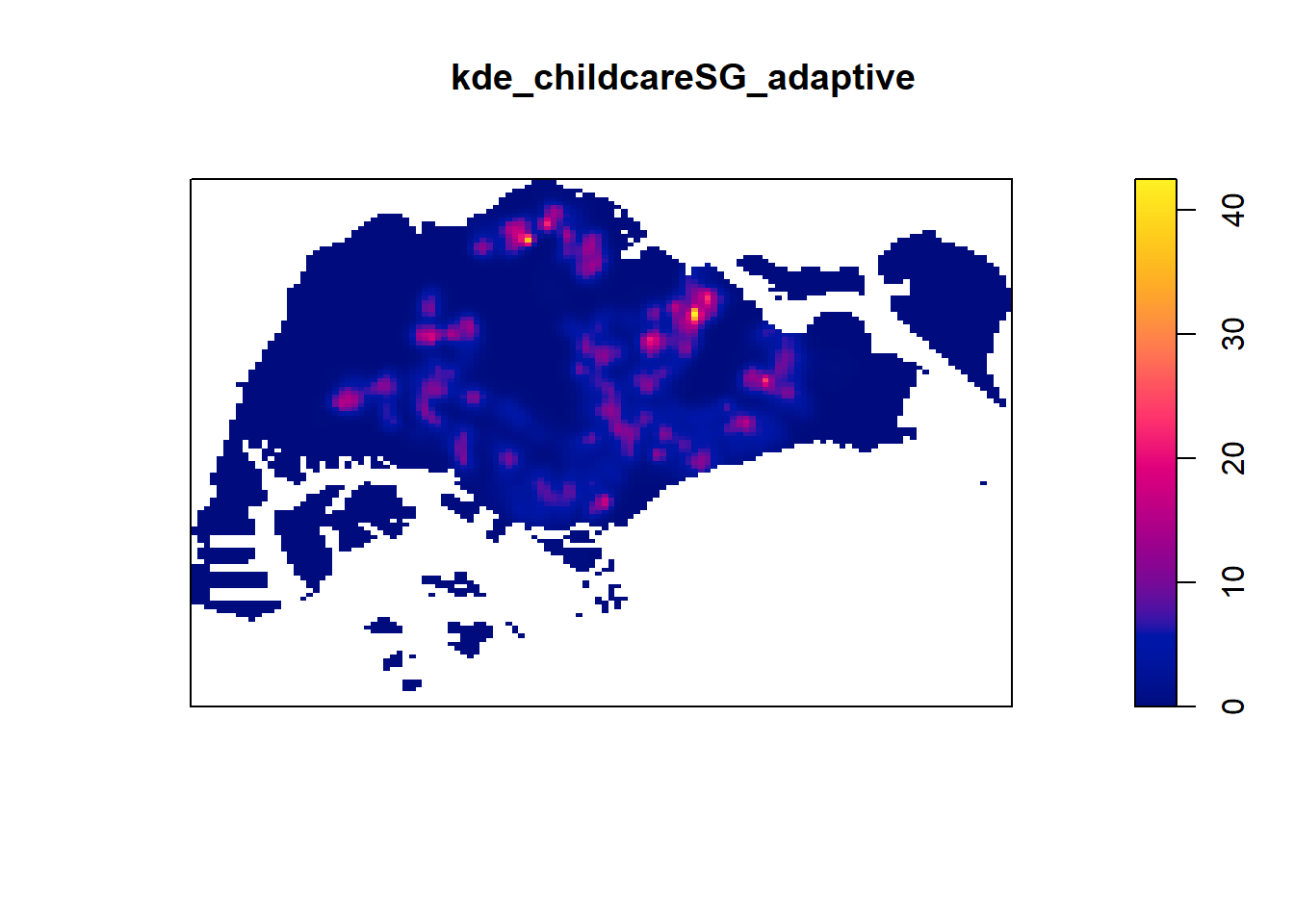
Kernel Density Estimation
par(bg = '#E4D5C9')

gridded_kde_childcareSG_ad <- maptools::as.SpatialGridDataFrame.im(
  kde_childcareSG_adaptive)
Please note that 'maptools' will be retired during October 2023,
plan transition at your earliest convenience (see
https://r-spatial.org/r/2023/05/15/evolution4.html and earlier blogs
for guidance);some functionality will be moved to 'sp'.
Checking rgeos availability: FALSEspplot(gridded_kde_childcareSG_ad)
gridded_kde_childcareSG_ad <- as(
  kde_childcareSG_adaptive,
  "SpatialGridDataFrame")
spplot(gridded_kde_childcareSG_ad)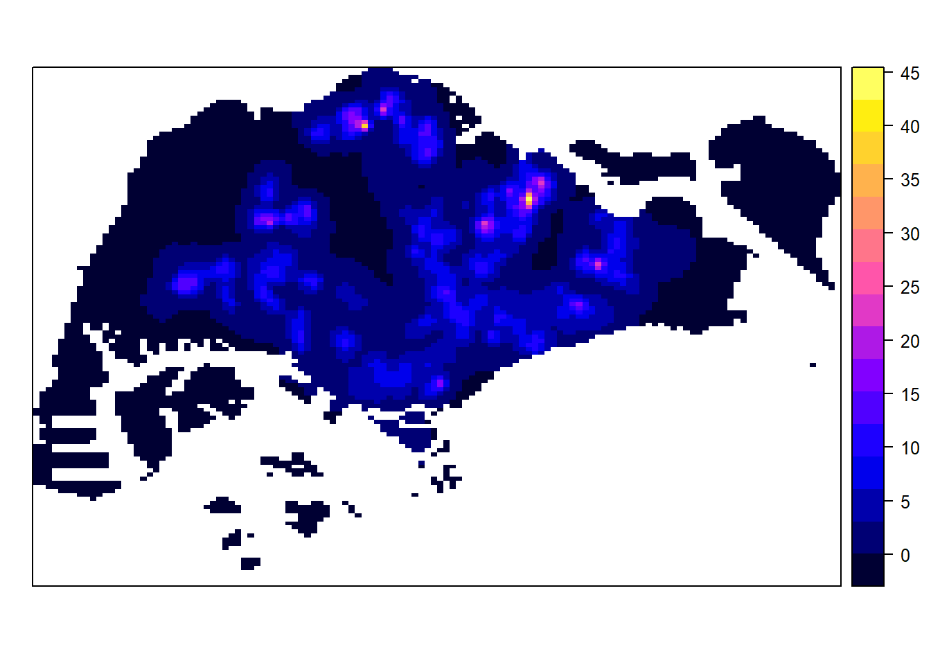
Kernel Density Estimation
Visualising KDE using tmap
kde_childcareSG_ad_raster <- raster(gridded_kde_childcareSG_ad)The code chunk below is used to plot the output raster by using tmap functions.
tm_shape(kde_childcareSG_ad_raster) +
  tm_raster(palette = "viridis") +
  tm_layout(legend.position = c("right", "bottom"),
            frame = FALSE,
            bg.color = "#E4D5C9")
Warning: Currect projection of shape kde_childcareSG_ad_raster unknown. Long
lat (epsg 4326) coordinates assumed.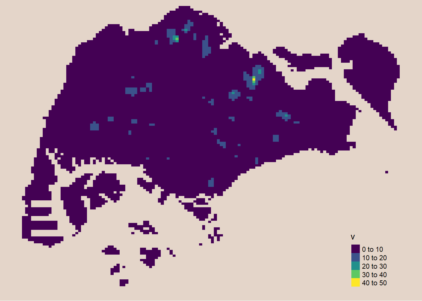
Extracting study area using sf objects
Extract and create an ppp object showing child care services and within Punggol Planning Area
On the other hand, filter() of dplyr package should be used to extract the target planning areas as shown in the code chunk below.
pg_owin <- mpsz_sf %>%
  filter(PLN_AREA_N == "PUNGGOL") %>%
  as.owin()

childcare_pg = childcare_ppp[pg_owin]

plot(childcare_pg)
Warning in default.charmap(ntypes, chars): Too many types to display every type
as a different characterWarning: Only 10 out of 61 symbols are shown in the symbol map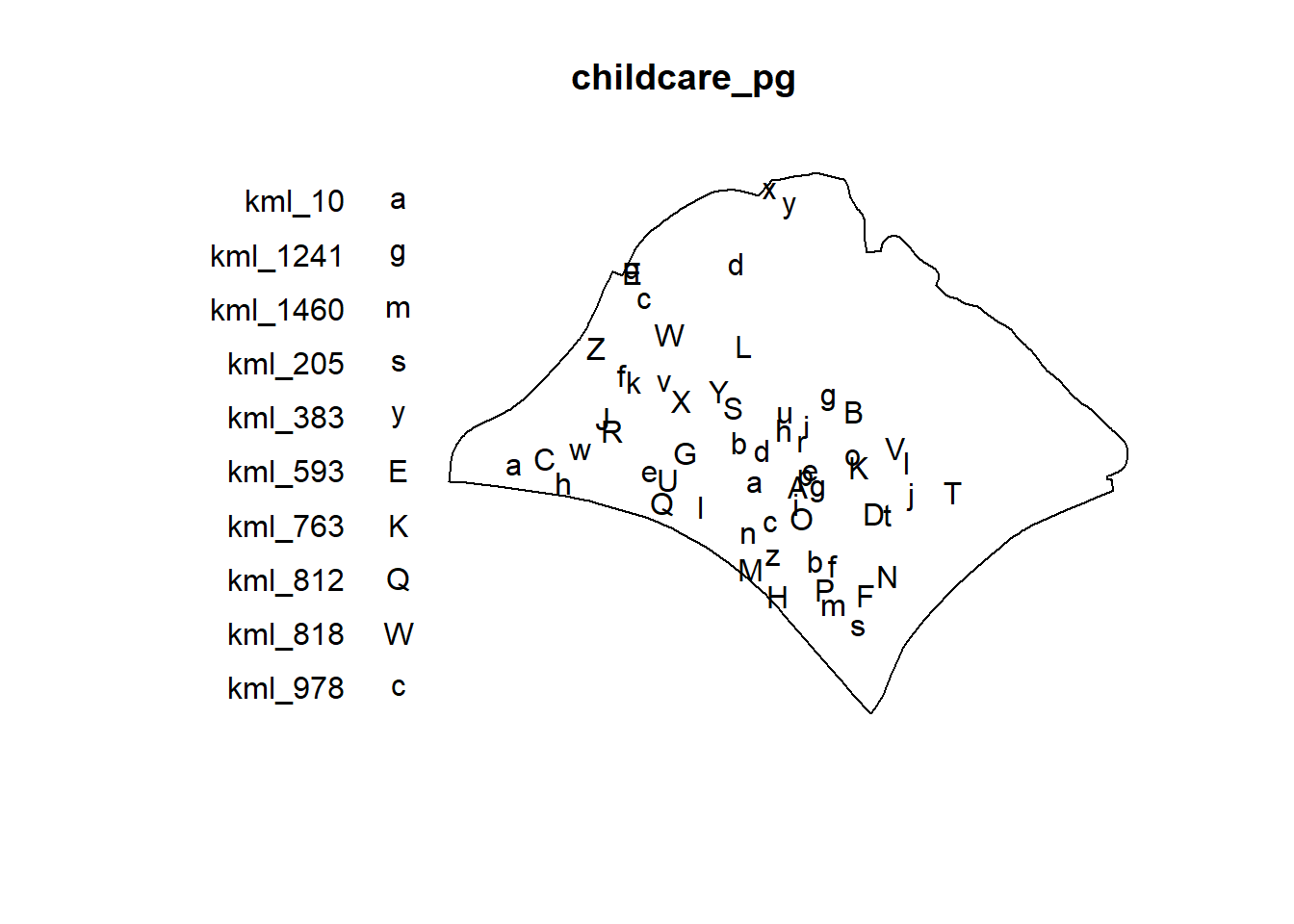
Monte Carlo Simulation
In order to ensure reproducibility, it is important to include the code chunk below before using spatstat functions involve Monte Carlo simulation.
set.seed(1234)Edge correction methods of spatstat
In spatstat, edge correction methods are used to handle biases that arise when estimating spatial statistics near the boundaries of a study region. These corrections are essential for ensuring accurate estimates in spatial point pattern analysis, especially for summary statistics like the K-function, L-function, pair correlation function, etc.
Common Edge Correction Methods in spatstat
“none”: No edge correction is applied. This method assumes that there is no bias at the edges, which may lead to underestimation of statistics near the boundaries.
“isotropic”: This method corrects for edge effects by assuming that the point pattern is isotropic (uniform in all directions). It compensates for missing neighbors outside the boundary by adjusting the distances accordingly.
“translate” (Translation Correction): This method uses a translation correction, which involves translating the observation window so that every point lies entirely within it. The statistic is then averaged over all possible translations.
“Ripley” (Ripley’s Correction): Similar to the isotropic correction but specifically tailored for Ripley’s K-function and related functions. It adjusts the expected number of neighbors for points near the edges based on the shape and size of the observation window.
“border”: Border correction reduces bias by only considering points far enough from the boundary so that their neighborhood is fully contained within the window. This can be quite conservative but reduces the influence of edge effects.