pacman::p_load(sf, raster, spatstat, tmap, tidyverse)Hands-on Exercise 2.2: 2nd Order Spatial Point Patterns Analysis Methods
1. Overview
Spatial Point Pattern Analysis is the evaluation of the pattern or distribution, of a set of points on a surface. The point can be location of:
events such as crime, traffic accident and disease onset, or
business services (coffee and fastfood outlets) or facilities such as childcare and eldercare.
Using appropriate functions of spatstat, this hands-on exercise aims to discover the spatial point processes of childecare centres in Singapore.
The specific questions we would like to answer are as follows:
are the childcare centres in Singapore randomly distributed throughout the country?
if the answer is not, then the next logical question is where are the locations with higher concentration of childcare centres?
2. Data
To provide answers to the questions above, three data sets will be used. They are:
CHILDCARE, a point feature data providing both location and attribute information of childcare centres. It was downloaded from Data.gov.sg and is in geojson format.MP14_SUBZONE_WEB_PL, a polygon feature data providing information of URA 2014 Master Plan Planning Subzone boundary data. It is in ESRI shapefile format. This data set was also downloaded from Data.gov.sg.CostalOutline, a polygon feature data showing the national boundary of Singapore. It is provided by SLA and is in ESRI shapefile format.
3. Installing and Loading the R packages
In this hands-on exercise, five R packages will be used, they are:
sf, a relatively new R package specially designed to import, manage and process vector-based geospatial data in R.
spatstat, which has a wide range of useful functions for point pattern analysis. In this hands-on exercise, it will be used to perform 1st- and 2nd-order spatial point patterns analysis and derive kernel density estimation (KDE) layer.
raster which reads, writes, manipulates, analyses and model of gridded spatial data (i.e. raster). In this hands-on exercise, it will be used to convert image output generate by spatstat into raster format.
maptools which provides a set of tools for manipulating geographic data. In this hands-on exercise, we mainly use it to convert Spatial objects into ppp format of spatstat.
tmap which provides functions for plotting cartographic quality static point patterns maps or interactive maps by using leaflet API.
Use the code chunk below to install and launch the five R packages.
4. Spatial Data Wrangling
4.1 Importing the spatial data
In this section, st_read() of sf package will be used to import these three geospatial data sets into R.
childcare_sf <- st_read("data/child-care-services-geojson.geojson") %>%
st_transform(crs = 3414)Reading layer `child-care-services-geojson' from data source
`C:\Users\user\OneDrive - Singapore Management University\MITB\6. Geospatial Analytics and Applications\jeffleesl\ISSS626-GAA\Hands-on_Ex\Hands-on_Ex02\data\child-care-services-geojson.geojson'
using driver `GeoJSON'
Simple feature collection with 1545 features and 2 fields
Geometry type: POINT
Dimension: XYZ
Bounding box: xmin: 103.6824 ymin: 1.248403 xmax: 103.9897 ymax: 1.462134
z_range: zmin: 0 zmax: 0
Geodetic CRS: WGS 84sg_sf <- st_read(dsn = "data", layer="CostalOutline")Reading layer `CostalOutline' from data source
`C:\Users\user\OneDrive - Singapore Management University\MITB\6. Geospatial Analytics and Applications\jeffleesl\ISSS626-GAA\Hands-on_Ex\Hands-on_Ex02\data'
using driver `ESRI Shapefile'
Simple feature collection with 60 features and 4 fields
Geometry type: POLYGON
Dimension: XY
Bounding box: xmin: 2663.926 ymin: 16357.98 xmax: 56047.79 ymax: 50244.03
Projected CRS: SVY21mpsz_sf <- st_read(dsn = "data",
layer = "MP14_SUBZONE_WEB_PL")Reading layer `MP14_SUBZONE_WEB_PL' from data source
`C:\Users\user\OneDrive - Singapore Management University\MITB\6. Geospatial Analytics and Applications\jeffleesl\ISSS626-GAA\Hands-on_Ex\Hands-on_Ex02\data'
using driver `ESRI Shapefile'
Simple feature collection with 323 features and 15 fields
Geometry type: MULTIPOLYGON
Dimension: XY
Bounding box: xmin: 2667.538 ymin: 15748.72 xmax: 56396.44 ymax: 50256.33
Projected CRS: SVY21Before we can use these data for analysis, it is important for us to ensure that they are projected in same projection system. undefined
sg_sf <- st_read(dsn = "data",
layer="CostalOutline") %>%
st_transform(crs = 3414)Reading layer `CostalOutline' from data source
`C:\Users\user\OneDrive - Singapore Management University\MITB\6. Geospatial Analytics and Applications\jeffleesl\ISSS626-GAA\Hands-on_Ex\Hands-on_Ex02\data'
using driver `ESRI Shapefile'
Simple feature collection with 60 features and 4 fields
Geometry type: POLYGON
Dimension: XY
Bounding box: xmin: 2663.926 ymin: 16357.98 xmax: 56047.79 ymax: 50244.03
Projected CRS: SVY21mpsz_sf <- st_read(dsn = "data",
layer = "MP14_SUBZONE_WEB_PL") %>%
st_transform(crs = 3414)Reading layer `MP14_SUBZONE_WEB_PL' from data source
`C:\Users\user\OneDrive - Singapore Management University\MITB\6. Geospatial Analytics and Applications\jeffleesl\ISSS626-GAA\Hands-on_Ex\Hands-on_Ex02\data'
using driver `ESRI Shapefile'
Simple feature collection with 323 features and 15 fields
Geometry type: MULTIPOLYGON
Dimension: XY
Bounding box: xmin: 2667.538 ymin: 15748.72 xmax: 56396.44 ymax: 50256.33
Projected CRS: SVY214.2 Mapping the geospatial data sets
After checking the referencing system of each geospatial data data frame, it is also useful for us to plot a map to show their spatial patterns.
tmap mode set to plotting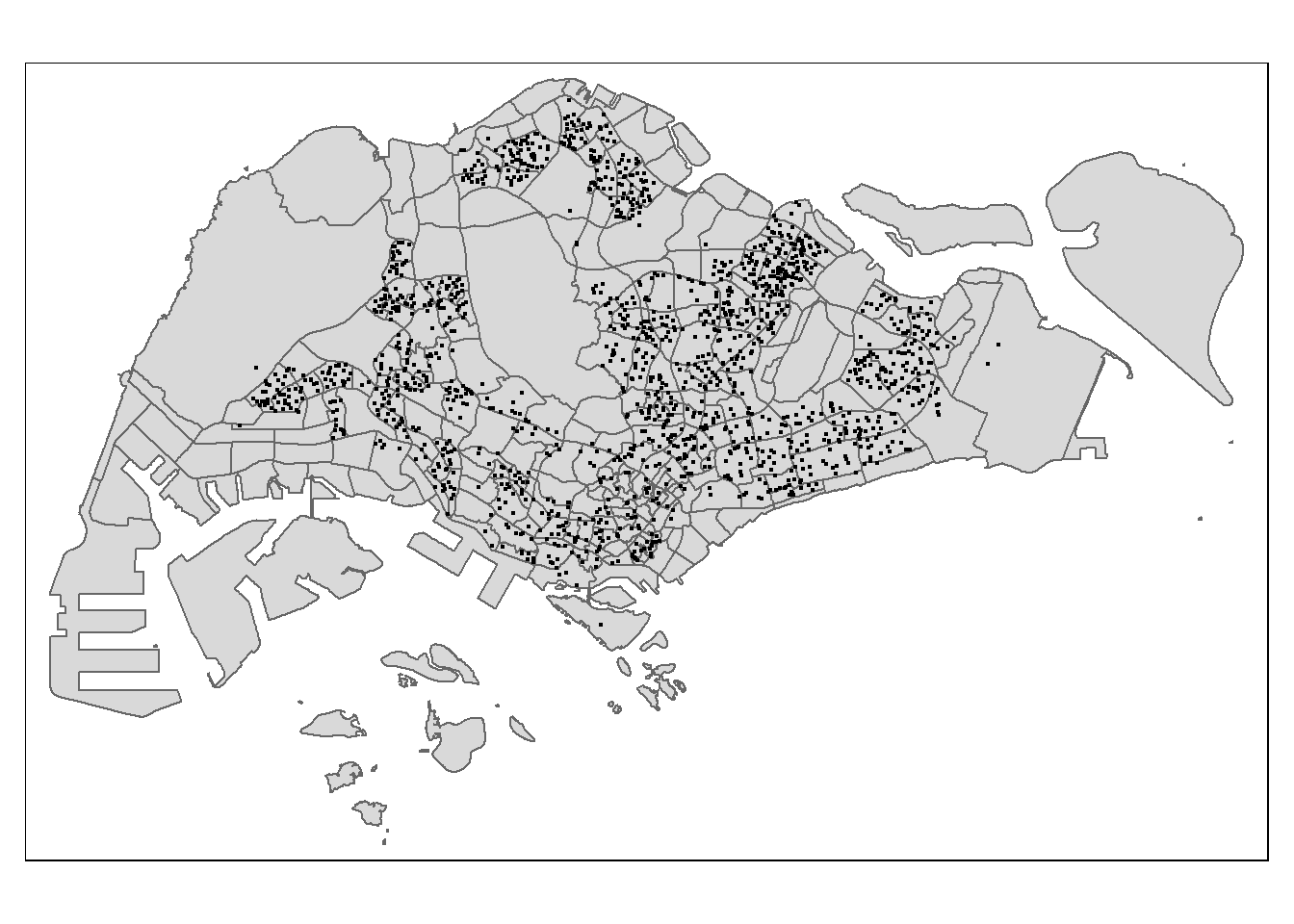
Notice that all the geospatial layers are within the same map extend. This shows that their referencing system and coordinate values are referred to similar spatial context. This is very important in any geospatial analysis.
Alternatively, we can also prepare a pin map by using the code chunk below.
tmap_mode('view')tmap mode set to interactive viewingtm_shape(childcare_sf)+
tm_dots()tmap_mode('plot')tmap mode set to plottingNotice that at the interactive mode, tmap is using leaflet for R API. The advantage of this interactive pin map is it allows us to navigate and zoom around the map freely. We can also query the information of each simple feature (i.e. the point) by clicking of them. Last but not least, you can also change the background of the internet map layer. Currently, three internet map layers are provided. They are: ESRI.WorldGrayCanvas, OpenStreetMap, and ESRI.WorldTopoMap. The default is ESRI.WorldGrayCanvas.
5. Geospatial Data wrangling
Although simple feature data frame is gaining popularity again sp’s Spatial* classes, there are, however, many geospatial analysis packages require the input geospatial data in sp’s Spatial* classes. In this section, you will learn how to convert simple feature data frame to sp’s Spatial* class.
5.1 Converting from sf format into spatstat’s ppp format
Now, we will use as.ppp() function of spatstat to convert the spatial data into spatstat’s ppp object format.
childcare_ppp <- as.ppp(childcare_sf)Warning in as.ppp.sf(childcare_sf): only first attribute column is used for
markschildcare_pppMarked planar point pattern: 1545 points
marks are of storage type 'character'
window: rectangle = [11203.01, 45404.24] x [25667.6, 49300.88] unitsNow, let us plot childcare_ppp and examine the different.
plot(childcare_ppp)Warning in default.charmap(ntypes, chars): Too many types to display every type
as a different characterWarning: Only 10 out of 1545 symbols are shown in the symbol map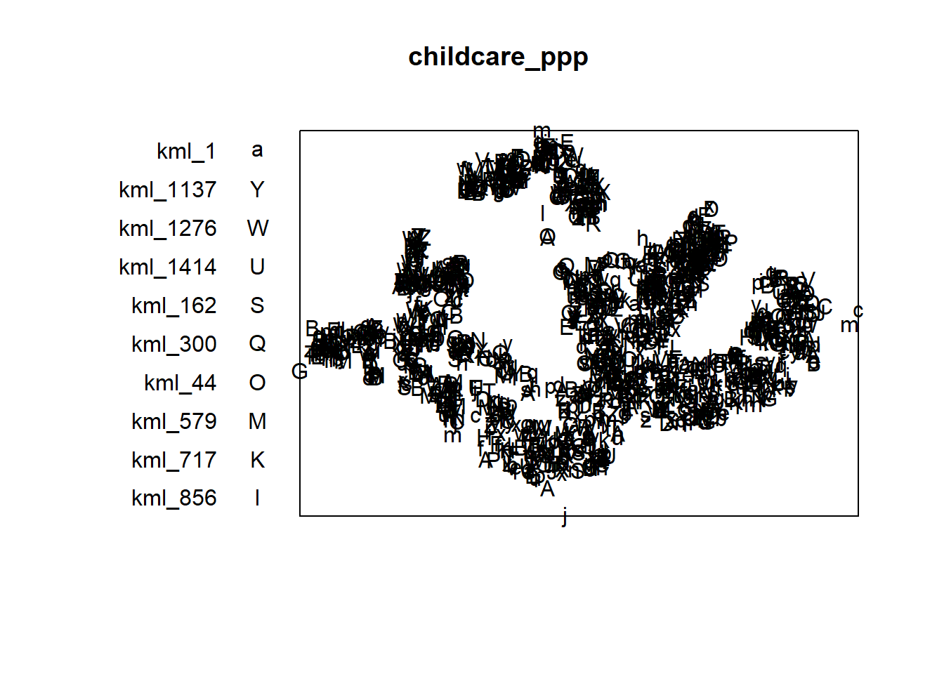
You can take a quick look at the summary statistics of the newly created ppp object by using the code chunk below.
summary(childcare_ppp)Marked planar point pattern: 1545 points
Average intensity 1.91145e-06 points per square unit
Coordinates are given to 11 decimal places
marks are of type 'character'
Summary:
Length Class Mode
1545 character character
Window: rectangle = [11203.01, 45404.24] x [25667.6, 49300.88] units
(34200 x 23630 units)
Window area = 808287000 square unitsNotice the warning message about duplicates. In spatial point patterns analysis an issue of significant is the presence of duplicates. The statistical methodology used for spatial point patterns processes is based largely on the assumption that process are simple, that is, that the points cannot be coincident.
5.2 Handling duplicated points
We can check the duplication in a ppp object by using the code chunk below.
any(duplicated(childcare_ppp))[1] FALSETo count the number of co-indicence point, we will use the multiplicity() function as shown in the code chunk below.
multiplicity(childcare_ppp) [1] 1 1 1 1 1 1 1 1 1 1 1 1 1 1 1 1 1 1 1 1 1 1 1 1 1 1 1 1 1 1 1 1 1 1 1 1 1
[38] 1 1 1 1 1 1 1 1 1 1 1 1 1 1 1 1 1 1 1 1 1 1 1 1 1 1 1 1 1 1 1 1 1 1 1 1 1
[75] 1 1 1 1 1 1 1 1 1 1 1 1 1 1 1 1 1 1 1 1 1 1 1 1 1 1 1 1 1 1 1 1 1 1 1 1 1
[112] 1 1 1 1 1 1 1 1 1 1 1 1 1 1 1 1 1 1 1 1 1 1 1 1 1 1 1 1 1 1 1 1 1 1 1 1 1
[149] 1 1 1 1 1 1 1 1 1 1 1 1 1 1 1 1 1 1 1 1 1 1 1 1 1 1 1 1 1 1 1 1 1 1 1 1 1
[186] 1 1 1 1 1 1 1 1 1 1 1 1 1 1 1 1 1 1 1 1 1 1 1 1 1 1 1 1 1 1 1 1 1 1 1 1 1
[223] 1 1 1 1 1 1 1 1 1 1 1 1 1 1 1 1 1 1 1 1 1 1 1 1 1 1 1 1 1 1 1 1 1 1 1 1 1
[260] 1 1 1 1 1 1 1 1 1 1 1 1 1 1 1 1 1 1 1 1 1 1 1 1 1 1 1 1 1 1 1 1 1 1 1 1 1
[297] 1 1 1 1 1 1 1 1 1 1 1 1 1 1 1 1 1 1 1 1 1 1 1 1 1 1 1 1 1 1 1 1 1 1 1 1 1
[334] 1 1 1 1 1 1 1 1 1 1 1 1 1 1 1 1 1 1 1 1 1 1 1 1 1 1 1 1 1 1 1 1 1 1 1 1 1
[371] 1 1 1 1 1 1 1 1 1 1 1 1 1 1 1 1 1 1 1 1 1 1 1 1 1 1 1 1 1 1 1 1 1 1 1 1 1
[408] 1 1 1 1 1 1 1 1 1 1 1 1 1 1 1 1 1 1 1 1 1 1 1 1 1 1 1 1 1 1 1 1 1 1 1 1 1
[445] 1 1 1 1 1 1 1 1 1 1 1 1 1 1 1 1 1 1 1 1 1 1 1 1 1 1 1 1 1 1 1 1 1 1 1 1 1
[482] 1 1 1 1 1 1 1 1 1 1 1 1 1 1 1 1 1 1 1 1 1 1 1 1 1 1 1 1 1 1 1 1 1 1 1 1 1
[519] 1 1 1 1 1 1 1 1 1 1 1 1 1 1 1 1 1 1 1 1 1 1 1 1 1 1 1 1 1 1 1 1 1 1 1 1 1
[556] 1 1 1 1 1 1 1 1 1 1 1 1 1 1 1 1 1 1 1 1 1 1 1 1 1 1 1 1 1 1 1 1 1 1 1 1 1
[593] 1 1 1 1 1 1 1 1 1 1 1 1 1 1 1 1 1 1 1 1 1 1 1 1 1 1 1 1 1 1 1 1 1 1 1 1 1
[630] 1 1 1 1 1 1 1 1 1 1 1 1 1 1 1 1 1 1 1 1 1 1 1 1 1 1 1 1 1 1 1 1 1 1 1 1 1
[667] 1 1 1 1 1 1 1 1 1 1 1 1 1 1 1 1 1 1 1 1 1 1 1 1 1 1 1 1 1 1 1 1 1 1 1 1 1
[704] 1 1 1 1 1 1 1 1 1 1 1 1 1 1 1 1 1 1 1 1 1 1 1 1 1 1 1 1 1 1 1 1 1 1 1 1 1
[741] 1 1 1 1 1 1 1 1 1 1 1 1 1 1 1 1 1 1 1 1 1 1 1 1 1 1 1 1 1 1 1 1 1 1 1 1 1
[778] 1 1 1 1 1 1 1 1 1 1 1 1 1 1 1 1 1 1 1 1 1 1 1 1 1 1 1 1 1 1 1 1 1 1 1 1 1
[815] 1 1 1 1 1 1 1 1 1 1 1 1 1 1 1 1 1 1 1 1 1 1 1 1 1 1 1 1 1 1 1 1 1 1 1 1 1
[852] 1 1 1 1 1 1 1 1 1 1 1 1 1 1 1 1 1 1 1 1 1 1 1 1 1 1 1 1 1 1 1 1 1 1 1 1 1
[889] 1 1 1 1 1 1 1 1 1 1 1 1 1 1 1 1 1 1 1 1 1 1 1 1 1 1 1 1 1 1 1 1 1 1 1 1 1
[926] 1 1 1 1 1 1 1 1 1 1 1 1 1 1 1 1 1 1 1 1 1 1 1 1 1 1 1 1 1 1 1 1 1 1 1 1 1
[963] 1 1 1 1 1 1 1 1 1 1 1 1 1 1 1 1 1 1 1 1 1 1 1 1 1 1 1 1 1 1 1 1 1 1 1 1 1
[1000] 1 1 1 1 1 1 1 1 1 1 1 1 1 1 1 1 1 1 1 1 1 1 1 1 1 1 1 1 1 1 1 1 1 1 1 1 1
[1037] 1 1 1 1 1 1 1 1 1 1 1 1 1 1 1 1 1 1 1 1 1 1 1 1 1 1 1 1 1 1 1 1 1 1 1 1 1
[1074] 1 1 1 1 1 1 1 1 1 1 1 1 1 1 1 1 1 1 1 1 1 1 1 1 1 1 1 1 1 1 1 1 1 1 1 1 1
[1111] 1 1 1 1 1 1 1 1 1 1 1 1 1 1 1 1 1 1 1 1 1 1 1 1 1 1 1 1 1 1 1 1 1 1 1 1 1
[1148] 1 1 1 1 1 1 1 1 1 1 1 1 1 1 1 1 1 1 1 1 1 1 1 1 1 1 1 1 1 1 1 1 1 1 1 1 1
[1185] 1 1 1 1 1 1 1 1 1 1 1 1 1 1 1 1 1 1 1 1 1 1 1 1 1 1 1 1 1 1 1 1 1 1 1 1 1
[1222] 1 1 1 1 1 1 1 1 1 1 1 1 1 1 1 1 1 1 1 1 1 1 1 1 1 1 1 1 1 1 1 1 1 1 1 1 1
[1259] 1 1 1 1 1 1 1 1 1 1 1 1 1 1 1 1 1 1 1 1 1 1 1 1 1 1 1 1 1 1 1 1 1 1 1 1 1
[1296] 1 1 1 1 1 1 1 1 1 1 1 1 1 1 1 1 1 1 1 1 1 1 1 1 1 1 1 1 1 1 1 1 1 1 1 1 1
[1333] 1 1 1 1 1 1 1 1 1 1 1 1 1 1 1 1 1 1 1 1 1 1 1 1 1 1 1 1 1 1 1 1 1 1 1 1 1
[1370] 1 1 1 1 1 1 1 1 1 1 1 1 1 1 1 1 1 1 1 1 1 1 1 1 1 1 1 1 1 1 1 1 1 1 1 1 1
[1407] 1 1 1 1 1 1 1 1 1 1 1 1 1 1 1 1 1 1 1 1 1 1 1 1 1 1 1 1 1 1 1 1 1 1 1 1 1
[1444] 1 1 1 1 1 1 1 1 1 1 1 1 1 1 1 1 1 1 1 1 1 1 1 1 1 1 1 1 1 1 1 1 1 1 1 1 1
[1481] 1 1 1 1 1 1 1 1 1 1 1 1 1 1 1 1 1 1 1 1 1 1 1 1 1 1 1 1 1 1 1 1 1 1 1 1 1
[1518] 1 1 1 1 1 1 1 1 1 1 1 1 1 1 1 1 1 1 1 1 1 1 1 1 1 1 1 1If we want to know how many locations have more than one point event, we can use the code chunk below.
sum(multiplicity(childcare_ppp) > 1)[1] 0The output shows that there are 128 duplicated point events.
To view the locations of these duplicate point events, we will plot childcare data by using the code chunk below.
tmap_mode('view')tmap mode set to interactive viewingtm_shape(childcare_sf) +
tm_dots(alpha=0.4,
size=0.05)tmap_mode('plot')tmap mode set to plottingThere are three ways to overcome this problem. The easiest way is to delete the duplicates. But, that will also mean that some useful point events will be lost.
The second solution is use jittering, which will add a small perturbation to the duplicate points so that they do not occupy the exact same space.
The third solution is to make each point “unique” and then attach the duplicates of the points to the patterns as marks, as attributes of the points. Then you would need analytical techniques that take into account these marks.
The code chunk below implements the jittering approach.
childcare_ppp_jit <- rjitter(childcare_ppp,
retry=TRUE,
nsim=1,
drop=TRUE)Check if any duplicated point in this geospatial data.
any(duplicated(childcare_ppp_jit))[1] FALSE5.3 Creating owin object
When analysing spatial point patterns, it is a good practice to confine the analysis with a geographical area like Singapore boundary. In spatstat, an object called owin is specially designed to represent this polygonal region.
The code chunk below is used to covert sg SpatialPolygon object into owin object of spatstat.
sg_owin <- as.owin(sg_sf)The ouput object can be displayed by using plot() function
plot(sg_owin)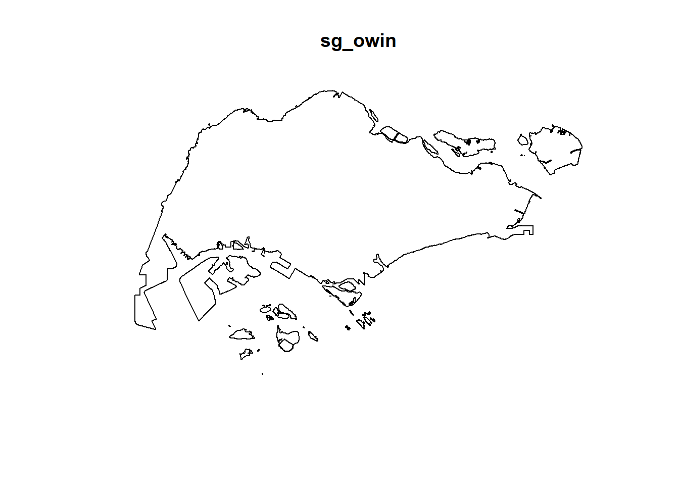
and summary() function of Base R.
summary(sg_owin)Window: polygonal boundary
50 separate polygons (1 hole)
vertices area relative.area
polygon 1 (hole) 30 -7081.18 -9.76e-06
polygon 2 55 82537.90 1.14e-04
polygon 3 90 415092.00 5.72e-04
polygon 4 49 16698.60 2.30e-05
polygon 5 38 24249.20 3.34e-05
polygon 6 976 23344700.00 3.22e-02
polygon 7 721 1927950.00 2.66e-03
polygon 8 1992 9992170.00 1.38e-02
polygon 9 330 1118960.00 1.54e-03
polygon 10 175 925904.00 1.28e-03
polygon 11 115 928394.00 1.28e-03
polygon 12 24 6352.39 8.76e-06
polygon 13 190 202489.00 2.79e-04
polygon 14 37 10170.50 1.40e-05
polygon 15 25 16622.70 2.29e-05
polygon 16 10 2145.07 2.96e-06
polygon 17 66 16184.10 2.23e-05
polygon 18 5195 636837000.00 8.78e-01
polygon 19 76 312332.00 4.31e-04
polygon 20 627 31891300.00 4.40e-02
polygon 21 20 32842.00 4.53e-05
polygon 22 42 55831.70 7.70e-05
polygon 23 67 1313540.00 1.81e-03
polygon 24 734 4690930.00 6.47e-03
polygon 25 16 3194.60 4.40e-06
polygon 26 15 4872.96 6.72e-06
polygon 27 15 4464.20 6.15e-06
polygon 28 14 5466.74 7.54e-06
polygon 29 37 5261.94 7.25e-06
polygon 30 111 662927.00 9.14e-04
polygon 31 69 56313.40 7.76e-05
polygon 32 143 145139.00 2.00e-04
polygon 33 397 2488210.00 3.43e-03
polygon 34 90 115991.00 1.60e-04
polygon 35 98 62682.90 8.64e-05
polygon 36 165 338736.00 4.67e-04
polygon 37 130 94046.50 1.30e-04
polygon 38 93 430642.00 5.94e-04
polygon 39 16 2010.46 2.77e-06
polygon 40 415 3253840.00 4.49e-03
polygon 41 30 10838.20 1.49e-05
polygon 42 53 34400.30 4.74e-05
polygon 43 26 8347.58 1.15e-05
polygon 44 74 58223.40 8.03e-05
polygon 45 327 2169210.00 2.99e-03
polygon 46 177 467446.00 6.44e-04
polygon 47 46 699702.00 9.65e-04
polygon 48 6 16841.00 2.32e-05
polygon 49 13 70087.30 9.66e-05
polygon 50 4 9459.63 1.30e-05
enclosing rectangle: [2663.93, 56047.79] x [16357.98, 50244.03] units
(53380 x 33890 units)
Window area = 725376000 square units
Fraction of frame area: 0.4015.4 Combining point events object and owin object
In this last step of geospatial data wrangling, we will extract childcare events that are located within Singapore by using the code chunk below.
childcareSG_ppp = childcare_ppp[sg_owin]The output object combined both the point and polygon feature in one ppp object class as shown below.
summary(childcareSG_ppp)Marked planar point pattern: 1545 points
Average intensity 2.129929e-06 points per square unit
Coordinates are given to 11 decimal places
marks are of type 'character'
Summary:
Length Class Mode
1545 character character
Window: polygonal boundary
50 separate polygons (1 hole)
vertices area relative.area
polygon 1 (hole) 30 -7081.18 -9.76e-06
polygon 2 55 82537.90 1.14e-04
polygon 3 90 415092.00 5.72e-04
polygon 4 49 16698.60 2.30e-05
polygon 5 38 24249.20 3.34e-05
polygon 6 976 23344700.00 3.22e-02
polygon 7 721 1927950.00 2.66e-03
polygon 8 1992 9992170.00 1.38e-02
polygon 9 330 1118960.00 1.54e-03
polygon 10 175 925904.00 1.28e-03
polygon 11 115 928394.00 1.28e-03
polygon 12 24 6352.39 8.76e-06
polygon 13 190 202489.00 2.79e-04
polygon 14 37 10170.50 1.40e-05
polygon 15 25 16622.70 2.29e-05
polygon 16 10 2145.07 2.96e-06
polygon 17 66 16184.10 2.23e-05
polygon 18 5195 636837000.00 8.78e-01
polygon 19 76 312332.00 4.31e-04
polygon 20 627 31891300.00 4.40e-02
polygon 21 20 32842.00 4.53e-05
polygon 22 42 55831.70 7.70e-05
polygon 23 67 1313540.00 1.81e-03
polygon 24 734 4690930.00 6.47e-03
polygon 25 16 3194.60 4.40e-06
polygon 26 15 4872.96 6.72e-06
polygon 27 15 4464.20 6.15e-06
polygon 28 14 5466.74 7.54e-06
polygon 29 37 5261.94 7.25e-06
polygon 30 111 662927.00 9.14e-04
polygon 31 69 56313.40 7.76e-05
polygon 32 143 145139.00 2.00e-04
polygon 33 397 2488210.00 3.43e-03
polygon 34 90 115991.00 1.60e-04
polygon 35 98 62682.90 8.64e-05
polygon 36 165 338736.00 4.67e-04
polygon 37 130 94046.50 1.30e-04
polygon 38 93 430642.00 5.94e-04
polygon 39 16 2010.46 2.77e-06
polygon 40 415 3253840.00 4.49e-03
polygon 41 30 10838.20 1.49e-05
polygon 42 53 34400.30 4.74e-05
polygon 43 26 8347.58 1.15e-05
polygon 44 74 58223.40 8.03e-05
polygon 45 327 2169210.00 2.99e-03
polygon 46 177 467446.00 6.44e-04
polygon 47 46 699702.00 9.65e-04
polygon 48 6 16841.00 2.32e-05
polygon 49 13 70087.30 9.66e-05
polygon 50 4 9459.63 1.30e-05
enclosing rectangle: [2663.93, 56047.79] x [16357.98, 50244.03] units
(53380 x 33890 units)
Window area = 725376000 square units
Fraction of frame area: 0.401Plot the newly derived childcareSG_ppp as shown below
plot(childcareSG_ppp)Warning in default.charmap(ntypes, chars): Too many types to display every type
as a different characterWarning: Only 10 out of 1545 symbols are shown in the symbol map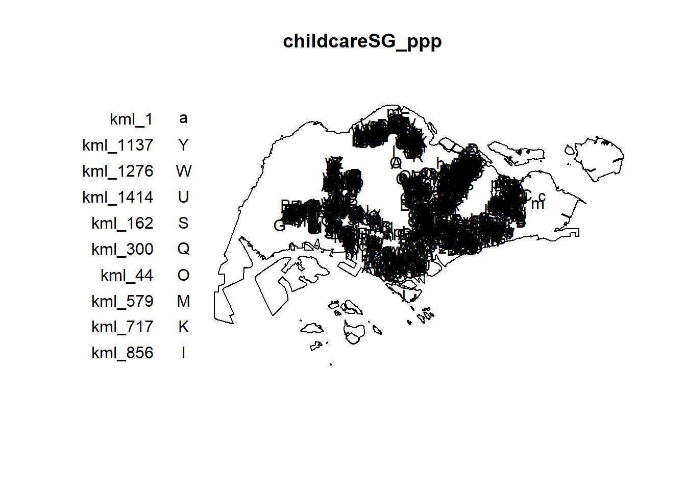
5.4.1 Extracting study area
The code chunk below will be used to extract the target planning areas.
pg <- mpsz_sf %>%
filter(PLN_AREA_N == "PUNGGOL")
tm <- mpsz_sf %>%
filter(PLN_AREA_N == "TAMPINES")
ck <- mpsz_sf %>%
filter(PLN_AREA_N == "CHOA CHU KANG")
jw <- mpsz_sf %>%
filter(PLN_AREA_N == "JURONG WEST")Plotting target planning areas
par(mfrow=c(2,2))
plot(pg, main = "Punggol")Warning: plotting the first 9 out of 15 attributes; use max.plot = 15 to plot
all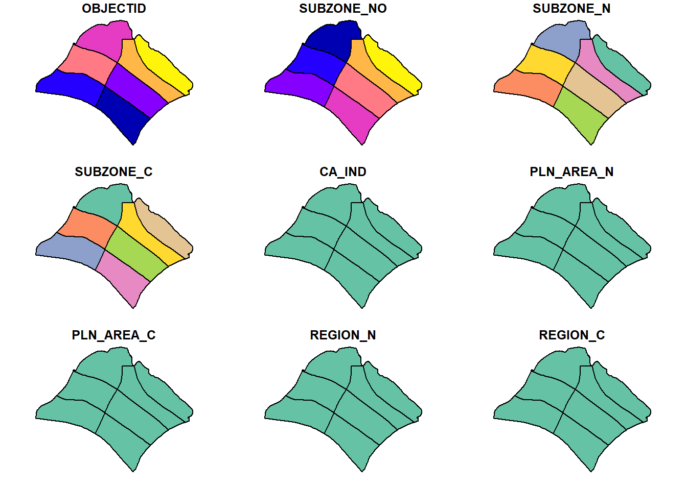
plot(tm, main = "Tampines")Warning: plotting the first 9 out of 15 attributes; use max.plot = 15 to plot
all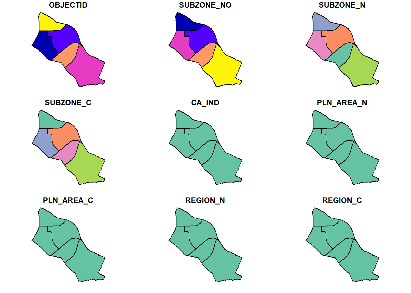
plot(ck, main = "Choa Chu Kang")Warning: plotting the first 10 out of 15 attributes; use max.plot = 15 to plot
all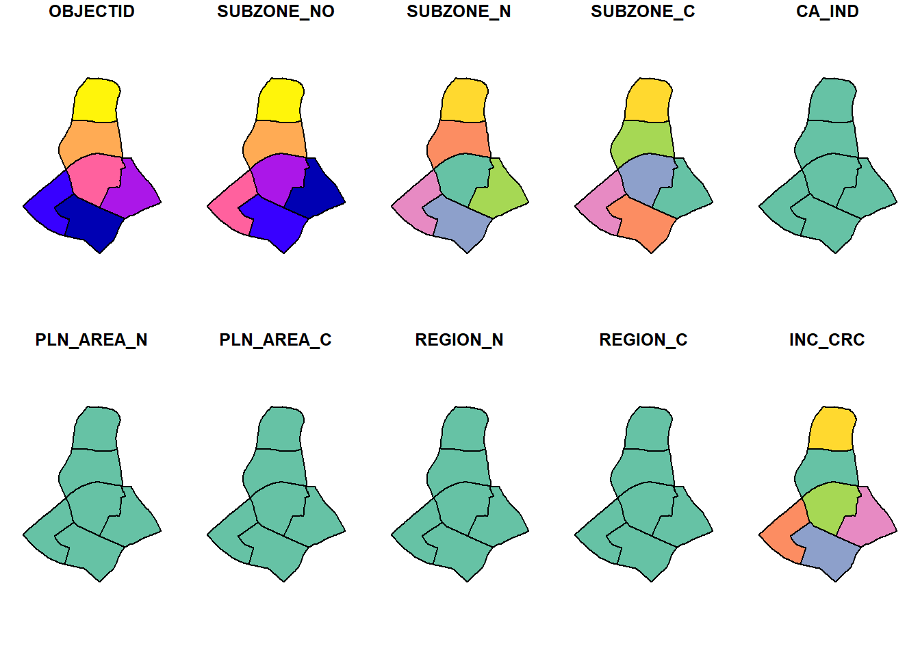
plot(jw, main = "Jurong West")Warning: plotting the first 9 out of 15 attributes; use max.plot = 15 to plot
all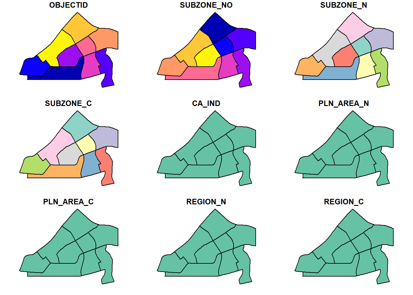
5.4.2 Converting sf objects into owin objects
Now, we will convert these sf objects into owin objects that is required by spatstat.
pg_owin = as.owin(pg)
tm_owin = as.owin(tm)
ck_owin = as.owin(ck)
jw_owin = as.owin(jw)5.4.3 Combining childcare points and the study area
By using the code chunk below, we are able to extract childcare that is within the specific region to do our analysis later on.
childcare_pg_ppp = childcare_ppp_jit[pg_owin]
childcare_tm_ppp = childcare_ppp_jit[tm_owin]
childcare_ck_ppp = childcare_ppp_jit[ck_owin]
childcare_jw_ppp = childcare_ppp_jit[jw_owin]Next, rescale() function is used to trasnform the unit of measurement from metre to kilometre.
childcare_pg_ppp.km = rescale(childcare_pg_ppp, 1000, "km")
childcare_tm_ppp.km = rescale(childcare_tm_ppp, 1000, "km")
childcare_ck_ppp.km = rescale(childcare_ck_ppp, 1000, "km")
childcare_jw_ppp.km = rescale(childcare_jw_ppp, 1000, "km")The code chunk below is used to plot these four study areas and the locations of the childcare centres.
par(mfrow=c(2,2))
plot(childcare_pg_ppp.km, main="Punggol")Warning in default.charmap(ntypes, chars): Too many types to display every type
as a different characterWarning: Only 10 out of 61 symbols are shown in the symbol mapplot(childcare_tm_ppp.km, main="Tampines")Warning in default.charmap(ntypes, chars): Too many types to display every type
as a different characterWarning: Only 10 out of 89 symbols are shown in the symbol mapplot(childcare_ck_ppp.km, main="Choa Chu Kang")Warning in default.charmap(ntypes, chars): Too many types to display every type
as a different characterWarning: Only 10 out of 61 symbols are shown in the symbol mapplot(childcare_jw_ppp.km, main="Jurong West")Warning in default.charmap(ntypes, chars): Too many types to display every type
as a different characterWarning: Only 10 out of 88 symbols are shown in the symbol map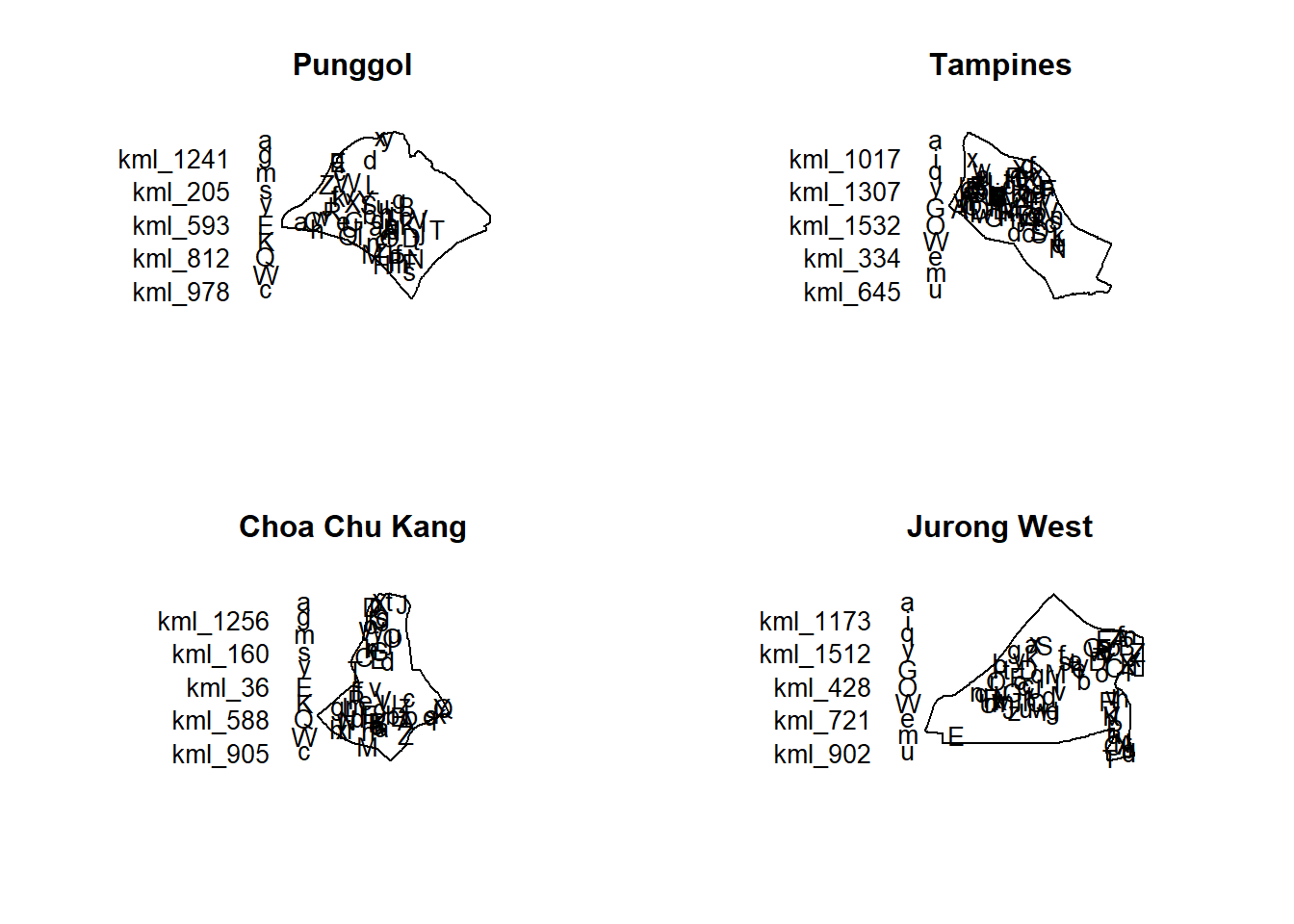
6. Second-order Spatial Point Patterns Analysis
7. Analysing Spatial Point Process Using G-Function
The G function measures the distribution of the distances from an arbitrary event to its nearest event. In this section, you will learn how to compute G-function estimation by using Gest() of spatstat package. You will also learn how to perform monta carlo simulation test using envelope() of spatstat package.
7.1 Choa Chu Kang planning area
7.1.1 Computing G-function estimation
The code chunk below is used to compute G-function using Gest() of spatat package.
G_CK = Gest(childcare_ck_ppp, correction = "border")
plot(G_CK, xlim=c(0,500))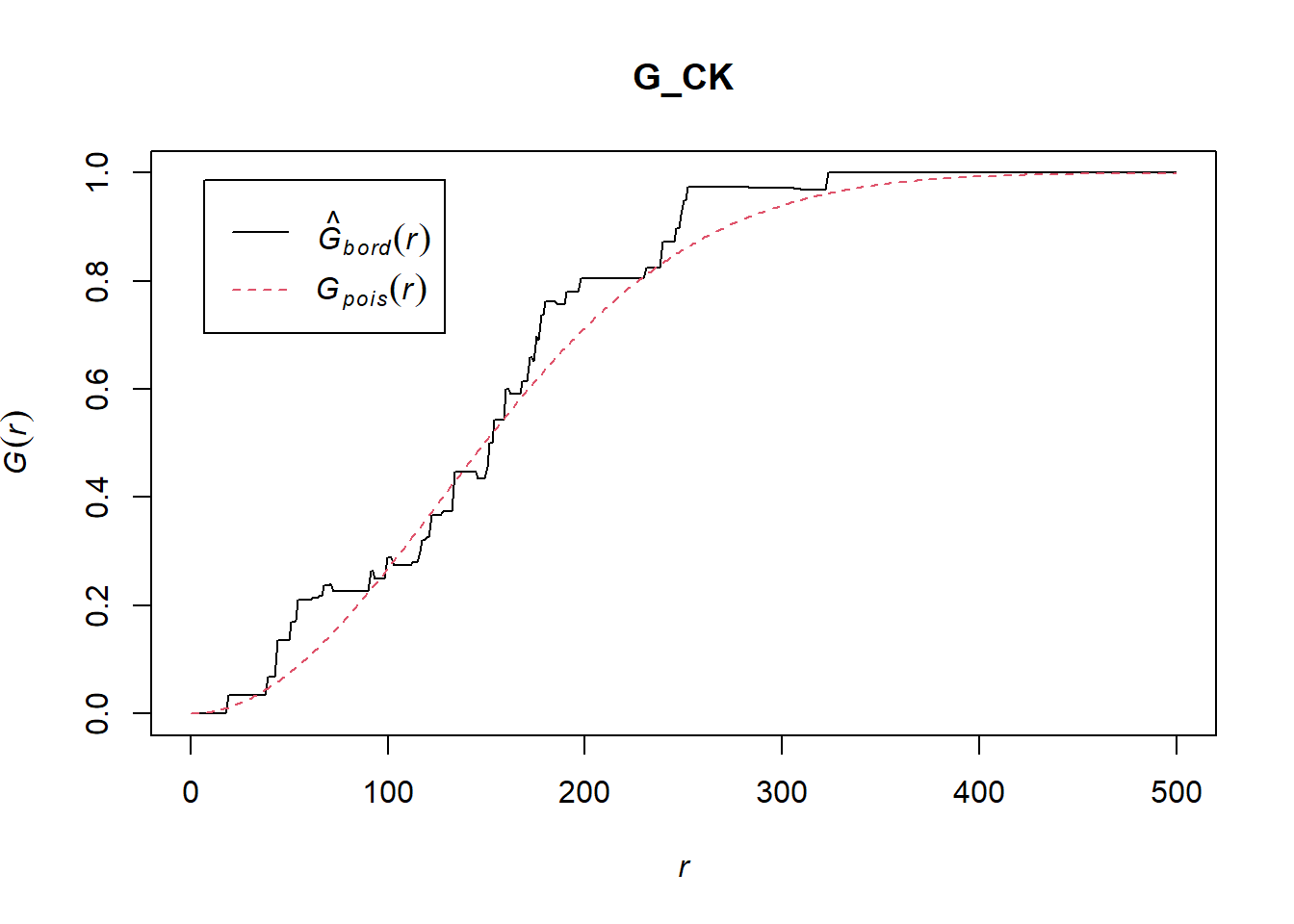
7.1.2 Performing Complete Spatial Randomness Test
To confirm the observed spatial patterns above, a hypothesis test will be conducted. The hypothesis and test are as follows:
Ho = The distribution of childcare services at Choa Chu Kang are randomly distributed.
H1= The distribution of childcare services at Choa Chu Kang are not randomly distributed.
The null hypothesis will be rejected if p-value is smaller than alpha value of 0.001.
Monte Carlo test with G-function
G_CK.csr <- envelope(childcare_ck_ppp, Gest, nsim = 999)Generating 999 simulations of CSR ...
1, 2, 3, ......10.........20.........30.........40.........50.........60..
.......70.........80.........90.........100.........110.........120.........130
.........140.........150.........160.........170.........180.........190........
.200.........210.........220.........230.........240.........250.........260......
...270.........280.........290.........300.........310.........320.........330....
.....340.........350.........360.........370.........380.........390.........400..
.......410.........420.........430.........440.........450.........460.........470
.........480.........490.........500.........510.........520.........530........
.540.........550.........560.........570.........580.........590.........600......
...610.........620.........630.........640.........650.........660.........670....
.....680.........690.........700.........710.........720.........730.........740..
.......750.........760.........770.........780.........790.........800.........810
.........820.........830.........840.........850.........860.........870........
.880.........890.........900.........910.........920.........930.........940......
...950.........960.........970.........980.........990........
999.
Done.plot(G_CK.csr)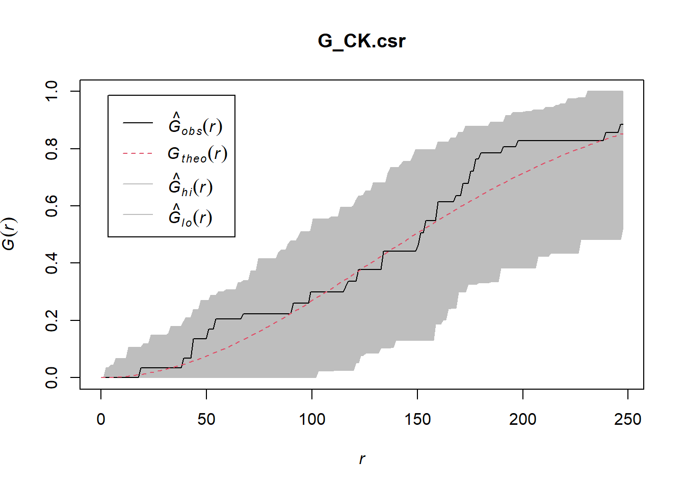
7.2 Tampines planning area
7.2.1 Computing G-function estimation
G_tm = Gest(childcare_tm_ppp, correction = "best")
plot(G_tm)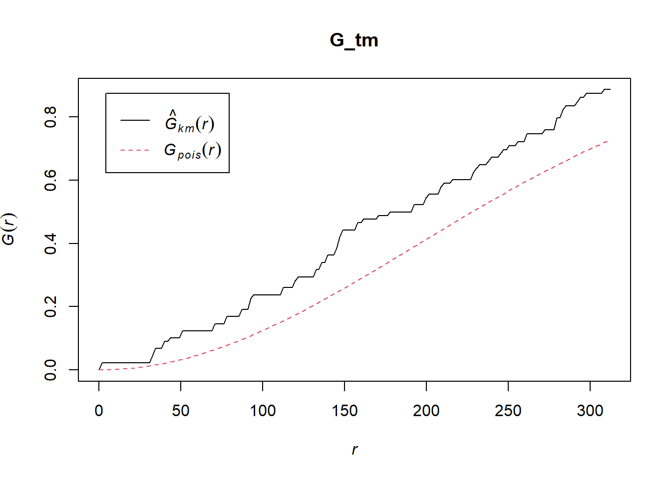
7.2.2 Performing Complete Spatial Randomness Test
To confirm the observed spatial patterns above, a hypothesis test will be conducted. The hypothesis and test are as follows:
Ho = The distribution of childcare services at Tampines are randomly distributed.
H1= The distribution of childcare services at Tampines are not randomly distributed.
The null hypothesis will be rejected is p-value is smaller than alpha value of 0.001.
The code chunk below is used to perform the hypothesis testing.
G_tm.csr <- envelope(childcare_tm_ppp, Gest, correction = "all", nsim = 999)Generating 999 simulations of CSR ...
1, 2, 3, ......10.........20.........30.........40.........50.........60..
.......70.........80.........90.........100.........110.........120.........130
.........140.........150.........160.........170.........180.........190........
.200.........210.........220.........230.........240.........250.........260......
...270.........280.........290.........300.........310.........320.........330....
.....340.........350.........360.........370.........380.........390.........400..
.......410.........420.........430.........440.........450.........460.........470
.........480.........490.........500.........510.........520.........530........
.540.........550.........560.........570.........580.........590.........600......
...610.........620.........630.........640.........650.........660.........670....
.....680.........690.........700.........710.........720.........730.........740..
.......750.........760.........770.........780.........790.........800.........810
.........820.........830.........840.........850.........860.........870........
.880.........890.........900.........910.........920.........930.........940......
...950.........960.........970.........980.........990........
999.
Done.plot(G_tm.csr)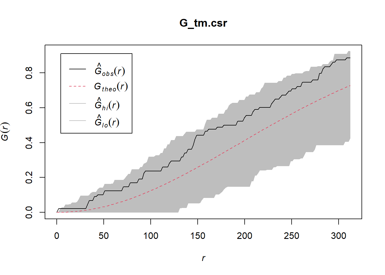
8. Analysing Spatial Point Process Using F-Function
The F function estimates the empty space function F(r) or its hazard rate h(r) from a point pattern in a window of arbitrary shape. In this section, you will learn how to compute F-function estimation by using Fest() of spatstat package. You will also learn how to perform monta carlo simulation test using envelope() of spatstat package.
8.1 Choa Chu Kang planning area
8.1.1 Computing F-function estimation
The code chunk below is used to compute F-function using Fest() of spatat package.
F_CK = Fest(childcare_ck_ppp)
plot(F_CK)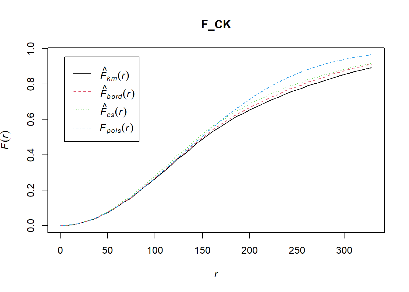
8.2 Performing Complete Spatial Randomness Test
To confirm the observed spatial patterns above, a hypothesis test will be conducted. The hypothesis and test are as follows:
Ho = The distribution of childcare services at Choa Chu Kang are randomly distributed.
H1= The distribution of childcare services at Choa Chu Kang are not randomly distributed.
The null hypothesis will be rejected if p-value is smaller than alpha value of 0.001.
Monte Carlo test with F-fucntion
F_CK.csr <- envelope(childcare_ck_ppp, Fest, nsim = 999)Generating 999 simulations of CSR ...
1, 2, 3, ......10.........20.........30.........40.........50.........60..
.......70.........80.........90.........100.........110.........120.........130
.........140.........150.........160.........170.........180.........190........
.200.........210.........220.........230.........240.........250.........260......
...270.........280.........290.........300.........310.........320.........330....
.....340.........350.........360.........370.........380.........390.........400..
.......410.........420.........430.........440.........450.........460.........470
.........480.........490.........500.........510.........520.........530........
.540.........550.........560.........570.........580.........590.........600......
...610.........620.........630.........640.........650.........660.........670....
.....680.........690.........700.........710.........720.........730.........740..
.......750.........760.........770.........780.........790.........800.........810
.........820.........830.........840.........850.........860.........870........
.880.........890.........900.........910.........920.........930.........940......
...950.........960.........970.........980.........990........
999.
Done.plot(F_CK.csr)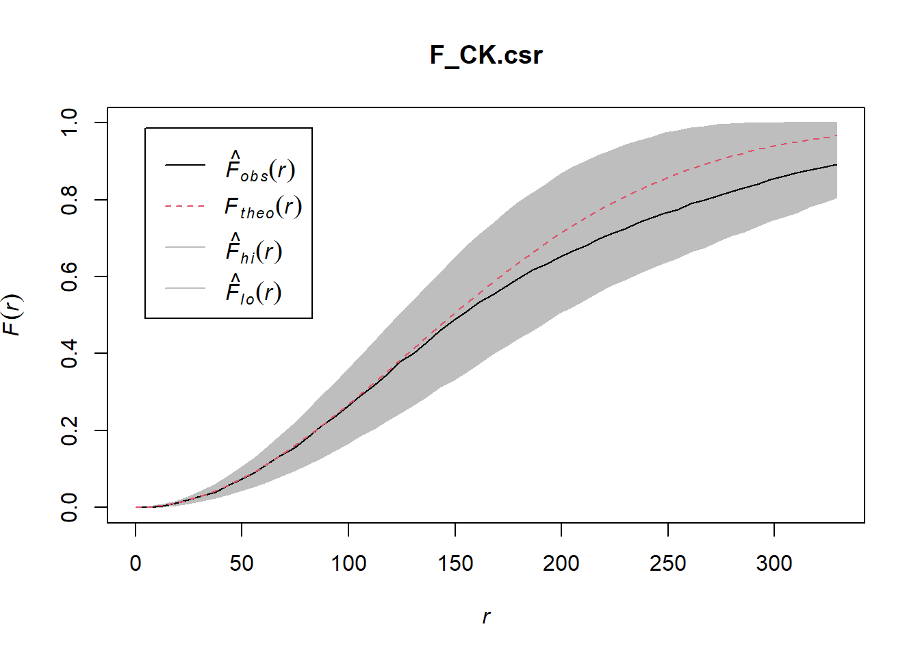
8.3 Tampines planning area
8.3.1 Computing F-function estimation
Monte Carlo test with F-fucntion
F_tm = Fest(childcare_tm_ppp, correction = "best")
plot(F_tm)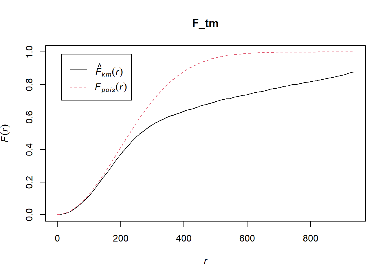
8.3.2 Performing Complete Spatial Randomness Test
To confirm the observed spatial patterns above, a hypothesis test will be conducted. The hypothesis and test are as follows:
Ho = The distribution of childcare services at Tampines are randomly distributed.
H1= The distribution of childcare services at Tampines are not randomly distributed.
The null hypothesis will be rejected is p-value is smaller than alpha value of 0.001.
The code chunk below is used to perform the hypothesis testing.
F_tm.csr <- envelope(childcare_tm_ppp, Fest, correction = "all", nsim = 999)Generating 999 simulations of CSR ...
1, 2, 3, ......10.........20.........30.........40.........50.........60..
.......70.........80.........90.........100.........110.........120.........130
.........140.........150.........160.........170.........180.........190........
.200.........210.........220.........230.........240.........250.........260......
...270.........280.........290.........300.........310.........320.........330....
.....340.........350.........360.........370.........380.........390.........400..
.......410.........420.........430.........440.........450.........460.........470
.........480.........490.........500.........510.........520.........530........
.540.........550.........560.........570.........580.........590.........600......
...610.........620.........630.........640.........650.........660.........670....
.....680.........690.........700.........710.........720.........730.........740..
.......750.........760.........770.........780.........790.........800.........810
.........820.........830.........840.........850.........860.........870........
.880.........890.........900.........910.........920.........930.........940......
...950.........960.........970.........980.........990........
999.
Done.plot(F_tm.csr)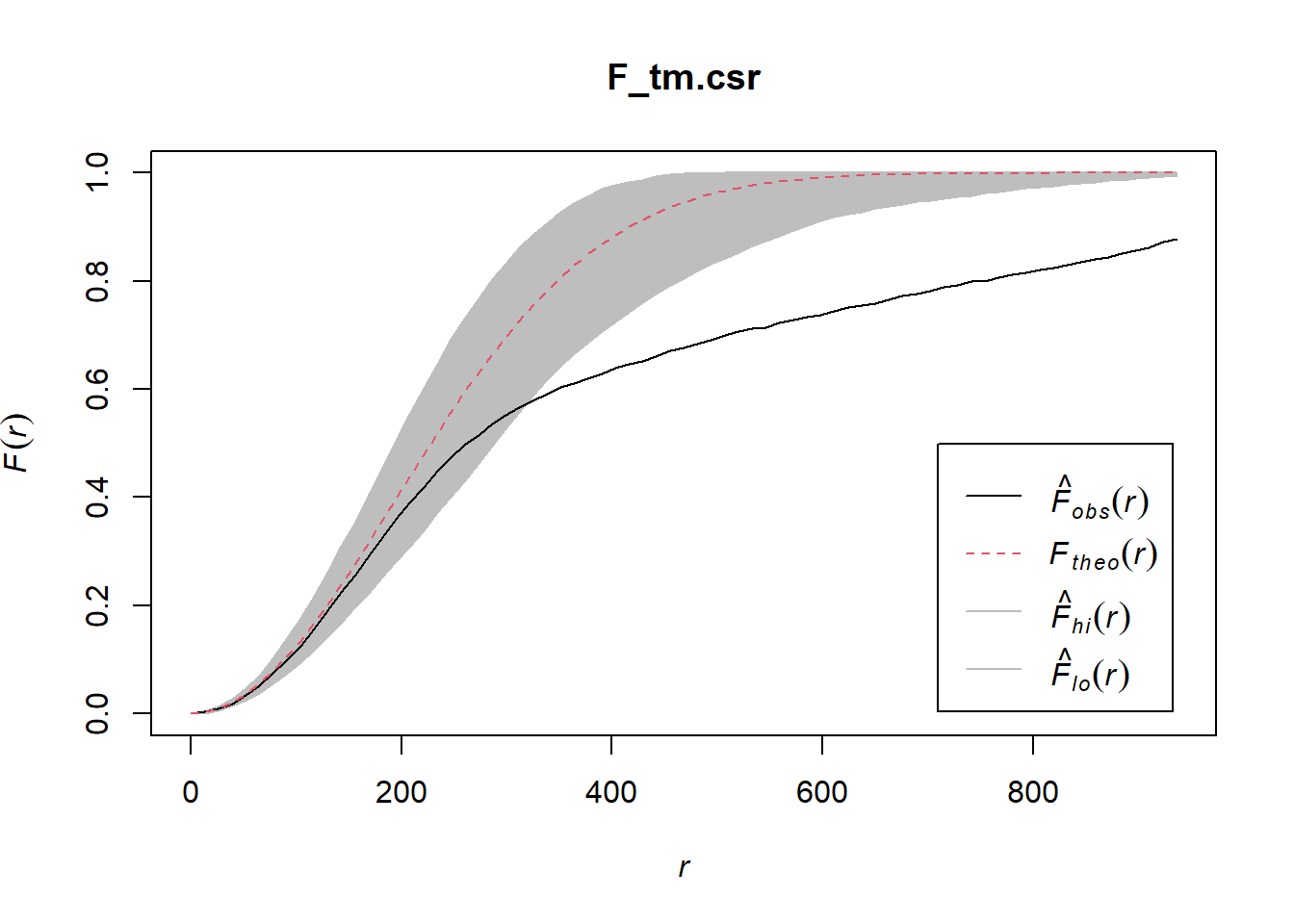
9. Analysing Spatial Point Process Using K-Function
K-function measures the number of events found up to a given distance of any particular event. In this section, you will learn how to compute K-function estimates by using Kest() of spatstat package. You will also learn how to perform monta carlo simulation test using envelope() of spatstat package.
9.1 Choa Chu Kang planning area
9.1.1 Computing K-fucntion estimate
K_ck = Kest(childcare_ck_ppp, correction = "Ripley")
plot(K_ck, . -r ~ r, ylab= "K(d)-r", xlab = "d(m)")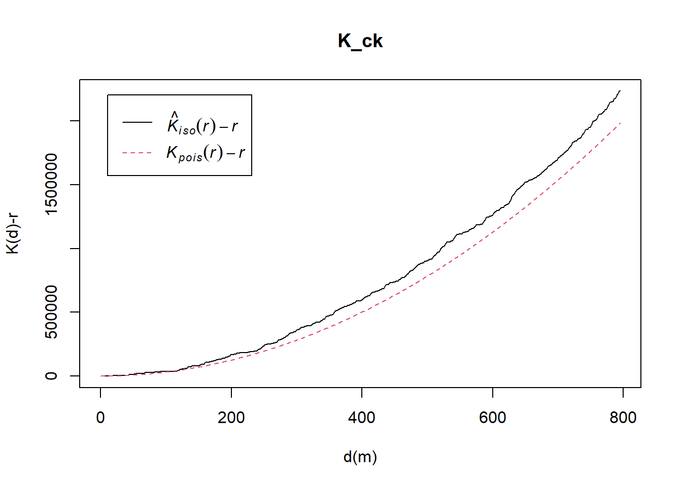
9.1.2 Performing Complete Spatial Randomness Test
To confirm the observed spatial patterns above, a hypothesis test will be conducted. The hypothesis and test are as follows:
Ho = The distribution of childcare services at Choa Chu Kang are randomly distributed.
H1= The distribution of childcare services at Choa Chu Kang are not randomly distributed.
The null hypothesis will be rejected if p-value is smaller than alpha value of 0.001.
The code chunk below is used to perform the hypothesis testing.
K_ck.csr <- envelope(childcare_ck_ppp, Kest, nsim = 99, rank = 1, glocal=TRUE)Generating 99 simulations of CSR ...
1, 2, 3, 4, 5, 6, 7, 8, 9, 10, 11, 12, 13, 14, 15, 16, 17, 18, 19, 20,
21, 22, 23, 24, 25, 26, 27, 28, 29, 30, 31, 32, 33, 34, 35, 36, 37, 38, 39, 40,
41, 42, 43, 44, 45, 46, 47, 48, 49, 50, 51, 52, 53, 54, 55, 56, 57, 58, 59, 60,
61, 62, 63, 64, 65, 66, 67, 68, 69, 70, 71, 72, 73, 74, 75, 76, 77, 78, 79, 80,
81, 82, 83, 84, 85, 86, 87, 88, 89, 90, 91, 92, 93, 94, 95, 96, 97, 98,
99.
Done.plot(K_ck.csr, . - r ~ r, xlab="d", ylab="K(d)-r")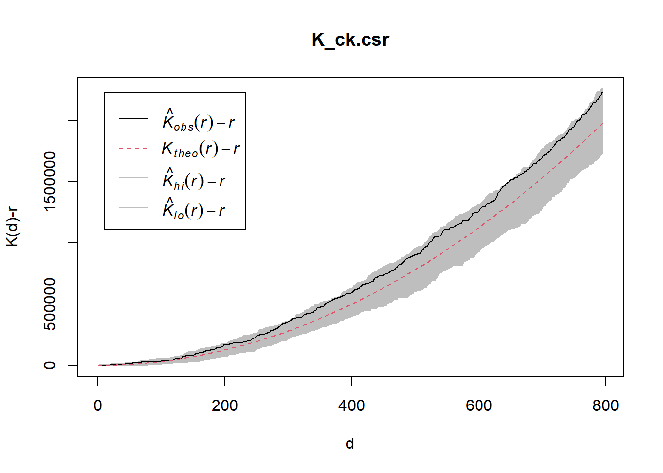
9.2 Tampines planning area
9.2.1 Computing K-fucntion estimation
K_tm = Kest(childcare_tm_ppp, correction = "Ripley")
plot(K_tm, . -r ~ r,
ylab= "K(d)-r", xlab = "d(m)",
xlim=c(0,1000))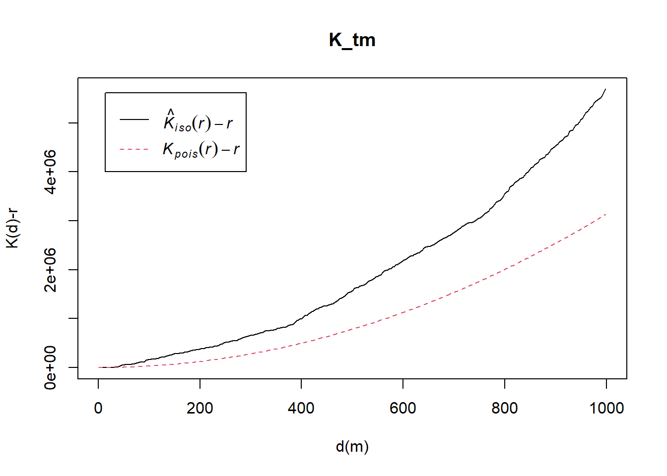
9.2.2 Performing Complete Spatial Randomness Test
To confirm the observed spatial patterns above, a hypothesis test will be conducted. The hypothesis and test are as follows:
Ho = The distribution of childcare services at Tampines are randomly distributed.
H1= The distribution of childcare services at Tampines are not randomly distributed.
The null hypothesis will be rejected if p-value is smaller than alpha value of 0.001.
The code chunk below is used to perform the hypothesis testing.
K_tm.csr <- envelope(childcare_tm_ppp, Kest, nsim = 99, rank = 1, glocal=TRUE)Generating 99 simulations of CSR ...
1, 2, 3, 4, 5, 6, 7, 8, 9, 10, 11, 12, 13, 14, 15, 16, 17, 18, 19, 20,
21, 22, 23, 24, 25, 26, 27, 28, 29, 30, 31, 32, 33, 34, 35, 36, 37, 38, 39, 40,
41, 42, 43, 44, 45, 46, 47, 48, 49, 50, 51, 52, 53, 54, 55, 56, 57, 58, 59, 60,
61, 62, 63, 64, 65, 66, 67, 68, 69, 70, 71, 72, 73, 74, 75, 76, 77, 78, 79, 80,
81, 82, 83, 84, 85, 86, 87, 88, 89, 90, 91, 92, 93, 94, 95, 96, 97, 98,
99.
Done.plot(K_tm.csr, . - r ~ r,
xlab="d", ylab="K(d)-r", xlim=c(0,500))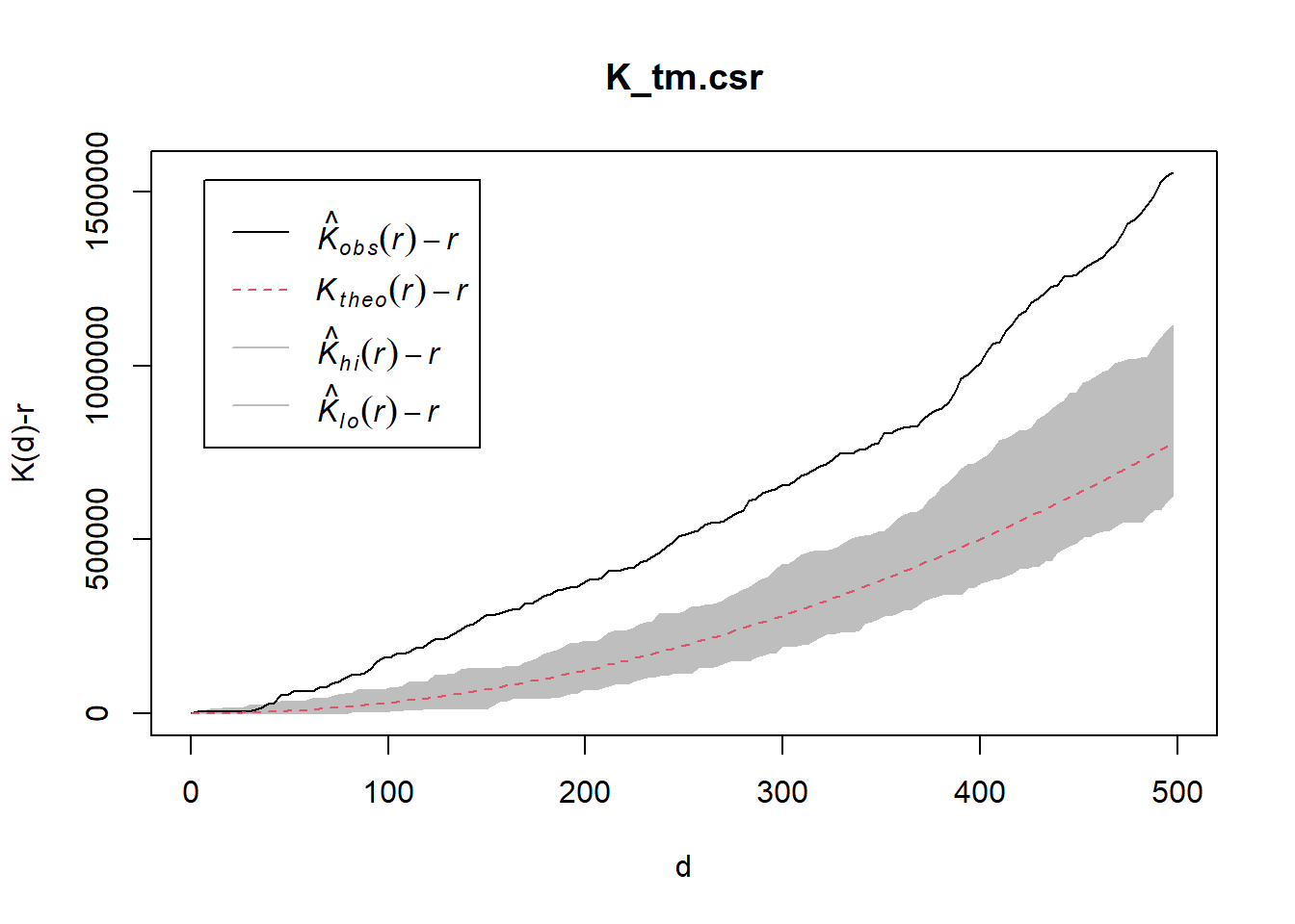
10. Analysing Spatial Point Process Using L-Function
In this section, you will learn how to compute L-function estimation by using Lest() of spatstat package. You will also learn how to perform monta carlo simulation test using envelope() of spatstat package.
10.1 Choa Chu Kang planning area
10.1.1 Computing L Function estimation
L_ck = Lest(childcare_ck_ppp, correction = "Ripley")
plot(L_ck, . -r ~ r,
ylab= "L(d)-r", xlab = "d(m)")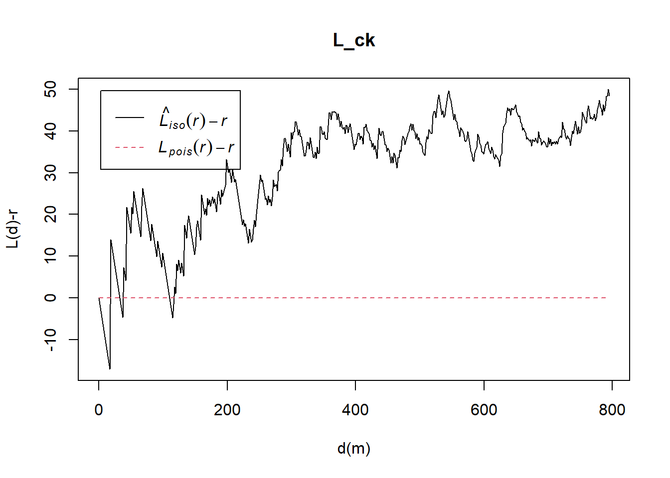
10.1.2 Performing Complete Spatial Randomness Test
To confirm the observed spatial patterns above, a hypothesis test will be conducted. The hypothesis and test are as follows:
Ho = The distribution of childcare services at Choa Chu Kang are randomly distributed.
H1= The distribution of childcare services at Choa Chu Kang are not randomly distributed.
The null hypothesis will be rejected if p-value if smaller than alpha value of 0.001.
The code chunk below is used to perform the hypothesis testing.
L_ck.csr <- envelope(childcare_ck_ppp, Lest, nsim = 99, rank = 1, glocal=TRUE)Generating 99 simulations of CSR ...
1, 2, 3, 4, 5, 6, 7, 8, 9, 10, 11, 12, 13, 14, 15, 16, 17, 18, 19, 20,
21, 22, 23, 24, 25, 26, 27, 28, 29, 30, 31, 32, 33, 34, 35, 36, 37, 38, 39, 40,
41, 42, 43, 44, 45, 46, 47, 48, 49, 50, 51, 52, 53, 54, 55, 56, 57, 58, 59, 60,
61, 62, 63, 64, 65, 66, 67, 68, 69, 70, 71, 72, 73, 74, 75, 76, 77, 78, 79, 80,
81, 82, 83, 84, 85, 86, 87, 88, 89, 90, 91, 92, 93, 94, 95, 96, 97, 98,
99.
Done.plot(L_ck.csr, . - r ~ r, xlab="d", ylab="L(d)-r")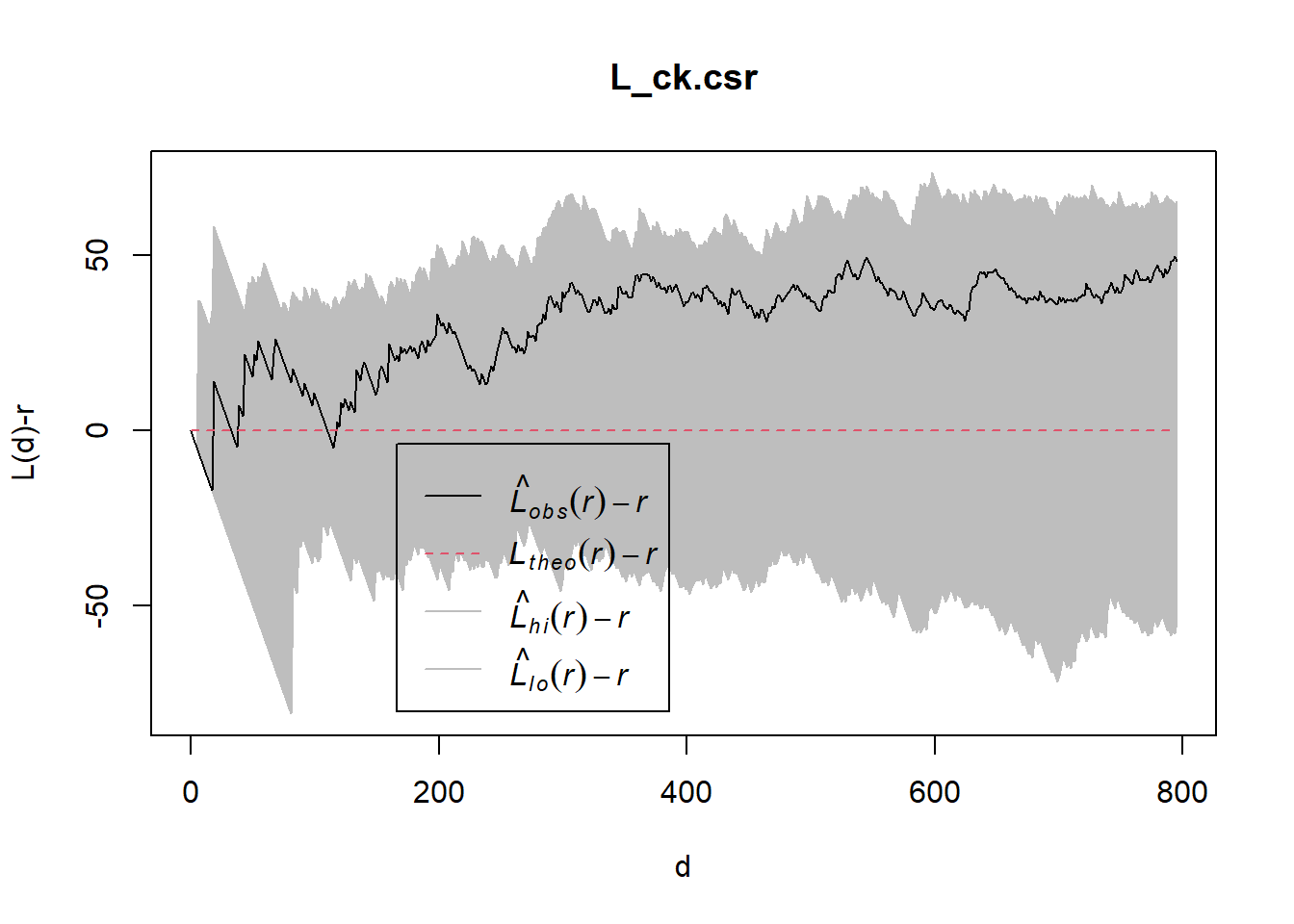
10.2 Tampines planning area
10.2.1 Computing L-fucntion estimate
L_tm = Lest(childcare_tm_ppp, correction = "Ripley")
plot(L_tm, . -r ~ r,
ylab= "L(d)-r", xlab = "d(m)",
xlim=c(0,1000))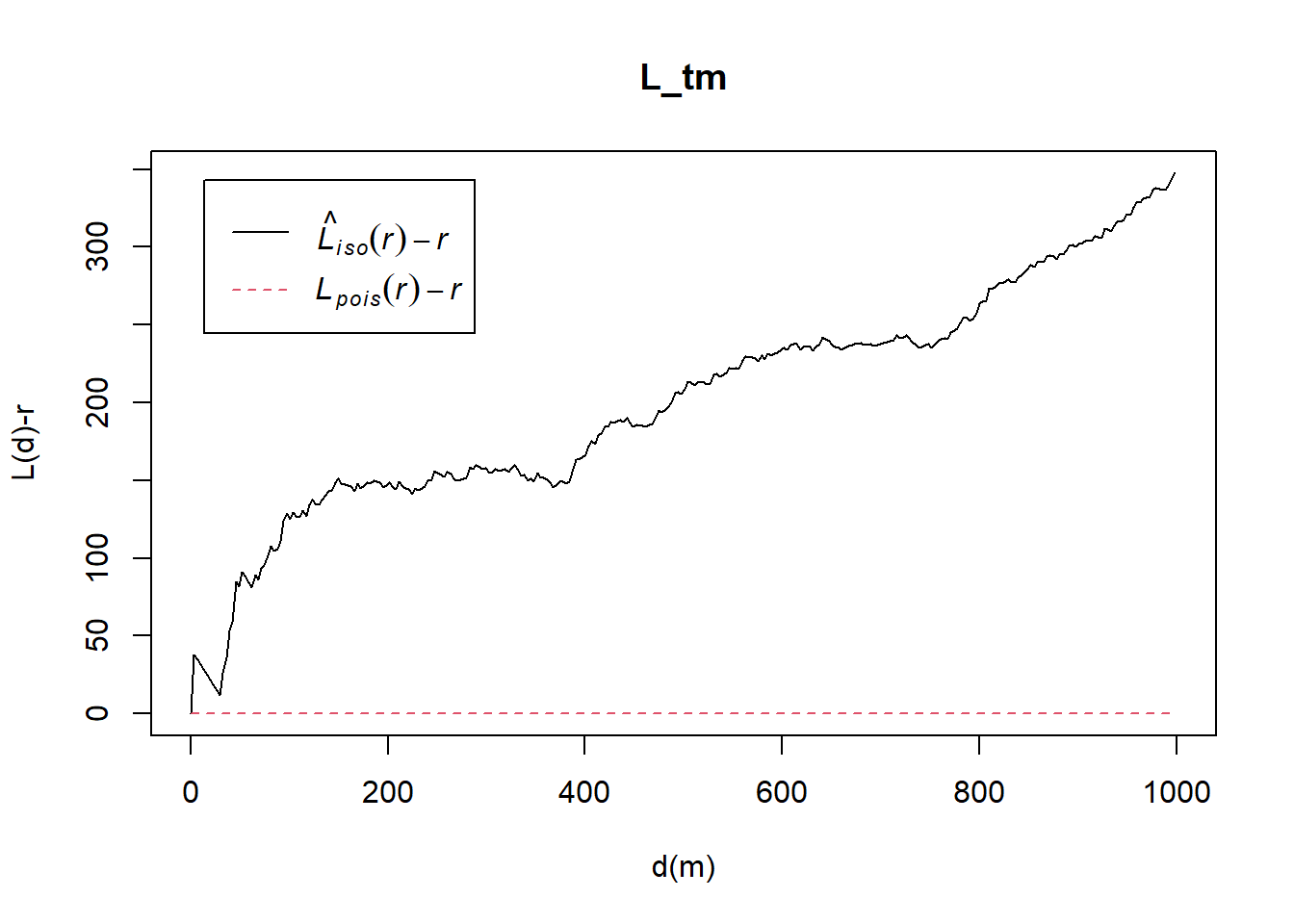
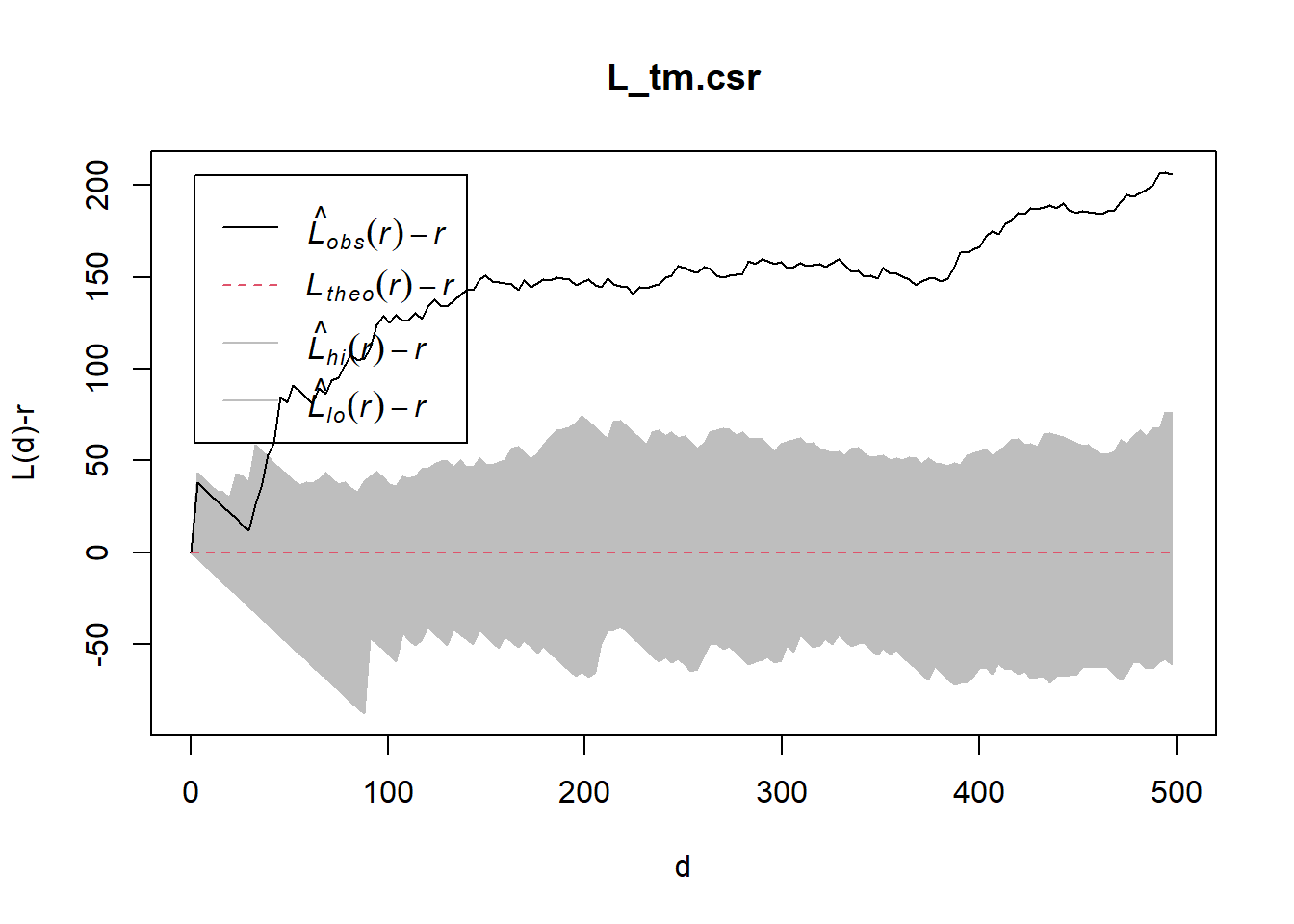
10.2.2 Performing Complete Spatial Randomness Test
To confirm the observed spatial patterns above, a hypothesis test will be conducted. The hypothesis and test are as follows:
Ho = The distribution of childcare services at Tampines are randomly distributed.
H1= The distribution of childcare services at Tampines are not randomly distributed.
The null hypothesis will be rejected if p-value is smaller than alpha value of 0.001.
The code chunk below will be used to perform the hypothesis testing.
L_tm.csr <- envelope(childcare_tm_ppp, Lest, nsim = 99, rank = 1, glocal=TRUE)Generating 99 simulations of CSR ...
1, 2, 3, 4, 5, 6, 7, 8, 9, 10, 11, 12, 13, 14, 15, 16, 17, 18, 19, 20,
21, 22, 23, 24, 25, 26, 27, 28, 29, 30, 31, 32, 33, 34, 35, 36, 37, 38, 39, 40,
41, 42, 43, 44, 45, 46, 47, 48, 49, 50, 51, 52, 53, 54, 55, 56, 57, 58, 59, 60,
61, 62, 63, 64, 65, 66, 67, 68, 69, 70, 71, 72, 73, 74, 75, 76, 77, 78, 79, 80,
81, 82, 83, 84, 85, 86, 87, 88, 89, 90, 91, 92, 93, 94, 95, 96, 97, 98,
99.
Done.Then, plot the model output by using the code chun below.
plot(L_tm.csr, . - r ~ r,
xlab="d", ylab="L(d)-r", xlim=c(0,500))