pacman::p_load(sf, sfdep, tmap, tidyverse)In-class Exercise 5: Global and Local Measures of Spatial Autocorrelation: sfdep methods
1. Introduction
Introducing sfdep.
sfdep creates an sf and tidyverse friendly interface to the package as well as introduces new functionality that is not present in spdep.
sfdep utilizes list columns extensively to make this interface possible.”
2. Getting started
Four R packages will be used for this in-class exercise, they are: sf, sfdep, tmap and tidyverse.
3. The Data
There are two data sets in this use case, they are:
Hunan, a geospatial data set in ESRI shapefile format, and
Hunan_2012, an attribute data set in csv format.
hunan <- st_read(dsn = "data/geospatial",
                 layer = "Hunan")
Reading layer `Hunan' from data source
`C:\Users\user\OneDrive - Singapore Management University\MITB\6. Geospatial Analytics and Applications\jeffleesl\ISSS626-GAA\In-class_Ex\In-class_Ex05\data\geospatial'
using driver `ESRI Shapefile'
Simple feature collection with 88 features and 7 fields
Geometry type: POLYGON
Dimension: XY
Bounding box: xmin: 108.7831 ymin: 24.6342 xmax: 114.2544 ymax: 30.12812
Geodetic CRS: WGS 844. Importing Attribute Table
hunan2012 <- read_csv("data/aspatial/Hunan_2012.csv")5. Combining both data frame by using left join
hunan_GDPPC <- left_join(hunan,hunan2012) %>%
  select(1:4, 7, 15)
Note
Note that there are five types of callouts, including: For the purpose of this exercise, we only retain column 1 to 4, column 7 and column 15. You should examine the output sf data.frame to learn know what are these fields.
Important
In order to retain the geospatial properties, the left data frame must the sf data.frame (i.e. hunan)
6. Plotting a choropleth map
Plot a choropleth map showing the distribution of GDPPC of Hunan Province.
tmap_mode("plot")
tm_shape(hunan_GDPPC) +
  tm_fill("GDPPC",
          style = "quantile",
          palette = "Blues",
          title = "GDPPC") +
  tm_borders(col = "grey") +
  tm_layout(main.title = "Distribution of GDP per capita by country, Hunan Province",
            main.title.position = "center",
            main.title.size = 1.2,
            legend.height = 0.45,
            legend.width = 0.35,
            frame = TRUE)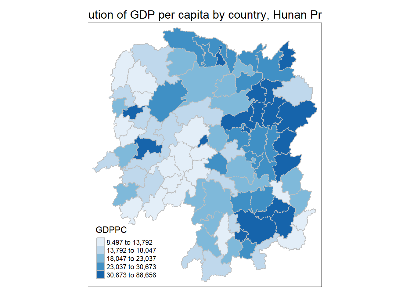
7. Global Measures of Spatial Association
7.1 Step 1: Deriving Queen’s contiguity weights: sfdep methods
wm_q <- hunan_GDPPC %>%
  mutate(nb = st_contiguity(geometry),
         wt = st_weights(nb,
                         style = "W"),
         .before = 1)
Notice that st_weights() provides tree arguments, they are:
nb: A neighbor list object as created by st_neighbors().
style: Default “W” for row standardized weights. This value can also be “B”, “C”, “U”, “minmax”, and “S”. B is the basic binary coding, W is row standardised (sums over all links to n), C is globally standardised (sums over all links to n), U is equal to C divided by the number of neighbours (sums over all links to unity), while S is the variance-stabilizing coding scheme proposed by Tiefelsdorf et al. 1999, p. 167-168 (sums over all links to n).
allow_zero: If TRUE, assigns zero as lagged value to zone without neighbors.
wm_qSimple feature collection with 88 features and 8 fields
Geometry type: POLYGON
Dimension: XY
Bounding box: xmin: 108.7831 ymin: 24.6342 xmax: 114.2544 ymax: 30.12812
Geodetic CRS: WGS 84
First 10 features:
nb
1 2, 3, 4, 57, 85
2 1, 57, 58, 78, 85
3 1, 4, 5, 85
4 1, 3, 5, 6
5 3, 4, 6, 85
6 4, 5, 69, 75, 85
7 67, 71, 74, 84
8 9, 46, 47, 56, 78, 80, 86
9 8, 66, 68, 78, 84, 86
10 16, 17, 19, 20, 22, 70, 72, 73
wt
1 0.2, 0.2, 0.2, 0.2, 0.2
2 0.2, 0.2, 0.2, 0.2, 0.2
3 0.25, 0.25, 0.25, 0.25
4 0.25, 0.25, 0.25, 0.25
5 0.25, 0.25, 0.25, 0.25
6 0.2, 0.2, 0.2, 0.2, 0.2
7 0.25, 0.25, 0.25, 0.25
8 0.1428571, 0.1428571, 0.1428571, 0.1428571, 0.1428571, 0.1428571, 0.1428571
9 0.1666667, 0.1666667, 0.1666667, 0.1666667, 0.1666667, 0.1666667
10 0.125, 0.125, 0.125, 0.125, 0.125, 0.125, 0.125, 0.125
NAME_2 ID_3 NAME_3 ENGTYPE_3 County GDPPC
1 Changde 21098 Anxiang County Anxiang 23667
2 Changde 21100 Hanshou County Hanshou 20981
3 Changde 21101 Jinshi County City Jinshi 34592
4 Changde 21102 Li County Li 24473
5 Changde 21103 Linli County Linli 25554
6 Changde 21104 Shimen County Shimen 27137
7 Changsha 21109 Liuyang County City Liuyang 63118
8 Changsha 21110 Ningxiang County Ningxiang 62202
9 Changsha 21111 Wangcheng County Wangcheng 70666
10 Chenzhou 21112 Anren County Anren 12761
geometry
1 POLYGON ((112.0625 29.75523...
2 POLYGON ((112.2288 29.11684...
3 POLYGON ((111.8927 29.6013,...
4 POLYGON ((111.3731 29.94649...
5 POLYGON ((111.6324 29.76288...
6 POLYGON ((110.8825 30.11675...
7 POLYGON ((113.9905 28.5682,...
8 POLYGON ((112.7181 28.38299...
9 POLYGON ((112.7914 28.52688...
10 POLYGON ((113.1757 26.82734...7.2 Computing Global Moran’ I
In the code chunk below, global_moran() function is used to compute the Moran’s I value. Different from spdep package, the output is a tibble data.frame.
moranI <- global_moran(wm_q$GDPPC,
                       wm_q$nb,
                       wm_q$wt)
glimpse(moranI)
List of 2
$ I: num 0.301
$ K: num 7.647.3 Performing Global Moran’sI test
In general, Moran’s I test will be performed instead of just computing the Moran’s I statistics. With sfdep package, Moran’s I test can be performed by using global_moran_test() as shown in the code chunk below.
global_moran_test(wm_q$GDPPC,
                  wm_q$nb,
                  wm_q$wt)
    Moran I test under randomisation

data:  x
weights: listw

Moran I statistic standard deviate = 4.7351, p-value = 1.095e-06
alternative hypothesis: greater
sample estimates:
Moran I statistic       Expectation          Variance
      0.300749970      -0.011494253       0.004348351
Tip
The default for
alternativeargument is “two.sided”. Other supported arguments are “greater” or “less”. randomization, andBy default the
randomizationargument is TRUE. If FALSE, under the assumption of normality.
7.4 Global Moran’I permutation test
In practice, Monte carlo simulation should be used to perform the statistical test. For sfdep, it is supported by globel_moran_perm()
It is always a good practice to use set.seed() before performing simulation. This is to ensure that the computation is reproducible.
set.seed(1234)Next, global_moran_perm() is used to perform Monte Carlo simulation.
global_moran_perm(wm_q$GDPPC,
                  wm_q$nb,
                  wm_q$wt,
                  nsim = 99)
    Monte-Carlo simulation of Moran I

data:  x
weights: listw
number of simulations + 1: 100

statistic = 0.30075, observed rank = 100, p-value < 2.2e-16
alternative hypothesis: two.sided
The statistical report on previous tab shows that the p-value is smaller than alpha value of 0.05. Hence, we have enough statistical evidence to reject the null hypothesis that the spatial distribution of GPD per capita are resemble random distribution (i.e. independent from spatial). Because the Moran’s I statistics is greater than 0. We can infer that the spatial distribution shows sign of clustering.
Reminder
The numbers of simulation is alway equal to nsim + 1. This mean in nsim = 99. This mean 100 simulation will be performed.
8. LISA map
LISA map is a categorical map showing outliers and clusters. There are two types of outliers namely: High-Low and Low-High outliers. Likewise, there are two type of clusters namely: High-High and Low-Low clusters. In fact, LISA map is an interpreted map by combining local Moran’s I of geographical areas and their respective p-values.
8.1 Computing local Moran’s I
In this section, you will learn how to compute Local Moran’s I of GDPPC at county level by using local_moran() of sfdep package.
lisa <- wm_q %>%
  mutate(local_moran = local_moran(
    GDPPC, nb, wt, nsim = 99),
    .before = 1) %>%
  unnest(local_moran)
The output of local_moran() is a sf data.frame containing the columns ii, eii, var_ii, z_ii, p_ii, p_ii_sim, and p_folded_sim.
ii: local moran statistic
eii: expectation of local moran statistic; for localmoran_permthe permutation sample means
var_ii: variance of local moran statistic; for localmoran_permthe permutation sample standard deviations
z_ii: standard deviate of local moran statistic; for localmoran_perm based on permutation sample means and standard deviations p_ii: p-value of local moran statistic using pnorm(); for localmoran_perm using standard deviatse based on permutation sample means and standard deviations p_ii_sim: For
localmoran_perm(),rank()andpunif()of observed statistic rank for [0, 1] p-values usingalternative=-p_folded_sim: the simulation folded [0, 0.5] range ranked p-value (based on https://github.com/pysal/esda/blob/4a63e0b5df1e754b17b5f1205b cadcbecc5e061/esda/crand.py#L211-L213)skewness: For
localmoran_perm, the output of e1071::skewness() for the permutation samples underlying the standard deviateskurtosis: For
localmoran_perm, the output of e1071::kurtosis() for the permutation samples underlying the standard deviates.
8.2 Visualising local Moran’s I
In this code chunk below, tmap functions are used prepare a choropleth map by using value in the ii field.
tmap_mode("plot")
tm_shape(lisa) +
  tm_fill("ii") +
  tm_borders(alpha = 0.5) +
  tm_view(set.zoom.limits = c(6,8)) +
  tm_layout(
    main.title = "local Moran's I of GDPPC",
    main.title.size = 2)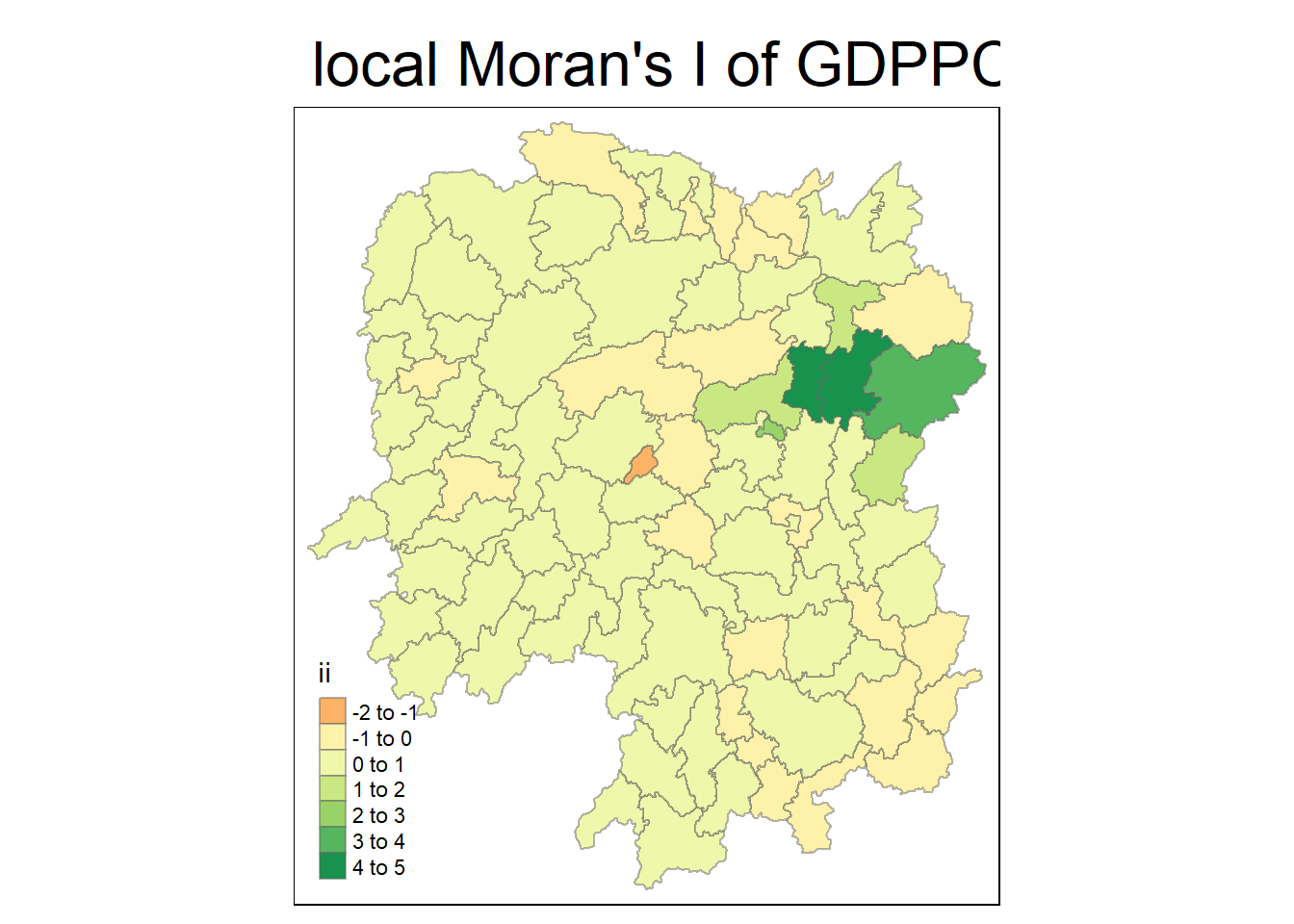
8.3 Visualising p-value of local Moran’s I
In the code chunk below, tmap functions are used prepare a choropleth map by using value in the p_ii_sim field.
tmap_mode("plot")
tm_shape(lisa) +
  tm_fill("p_ii_sim") +
  tm_borders(alpha = 0.5) +
  tm_layout(
    main.title = "p-values of local Moran's I",
    main.title.size = 2)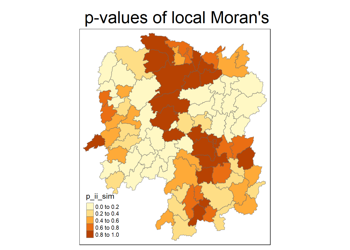
Warning
For p-values, the appropriate classification should be 0.001, 0.01, 0.05 and not significant instead of using default classification scheme.
8.4 Visualising local Moran’s I and p-value
tmap_mode("plot")
map1 <- tm_shape(lisa) +
  tm_fill("ii")+
  tm_borders(alpha=0.5)+
  tm_layout(main.title="p-value",
            main.title.size=2)

tmap_mode("plot")
map2 <- tm_shape(lisa) +
  tm_fill("p_ii_sim")+
  tm_borders(alpha=0.5)+
  tm_layout(main.title="p-value",
            main.title.size=2)

tmap_arrange(map1,
             map2,
             asp=1, #Aspect Ratio
             ncol=2)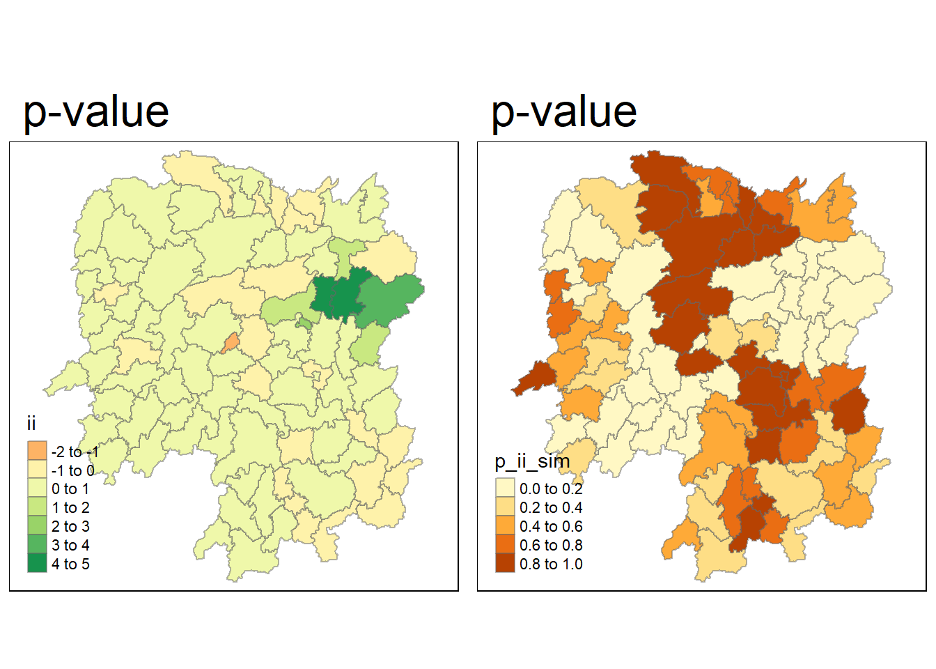
tmap_mode("plot")
map1 <- tm_shape(lisa) +
  tm_fill("ii") +
  tm_borders(alpha = 0.5) +
  tm_view(set.zoom.limits = c(6,8)) +
  tm_layout(main.title = "local Moran's I of GDPPC",
            main.title.size = 0.8)

map2 <- tm_shape(lisa) +
  tm_fill("p_ii",
          breaks = c(0, 0.001, 0.01, 0.05, 1),
              labels = c("0.001", "0.01", "0.05", "Not sig")) +
  tm_borders(alpha = 0.5) +
  tm_layout(main.title = "p-value of local Moran's I",
            main.title.size = 0.8)
tmap_arrange(map1, map2, ncol = 2)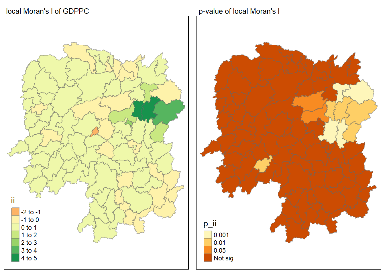
8.5 Plotting LISA map
In lisa sf data.frame, we can find three fields contain the LISA categories. They are mean, median and pysal. In general, classification in mean will be used as shown in the code chunk below.
lisa_sig <- lisa %>%
  filter(p_ii < 0.05) #filter only significant p values

tmap_mode("plot")
tm_shape(lisa)+
  tm_polygons()+
  tm_borders(alpha=0.5)+
tm_shape(lisa_sig)+
  tm_fill("mean")+
  tm_borders(alpha=0.4)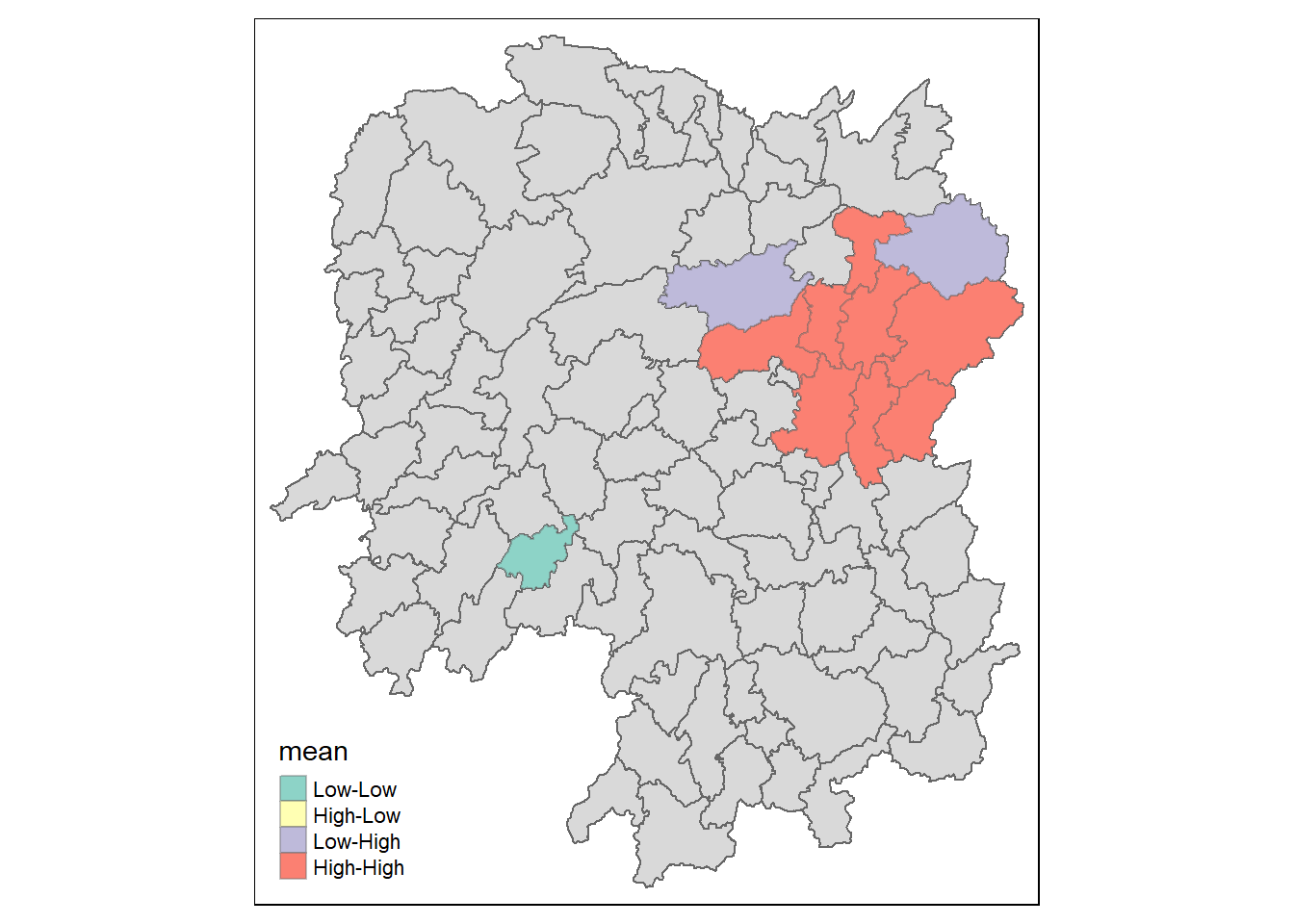
9. Hot Spot and Cold Spot Area Analysis (HCSA)
HCSA uses spatial weights to identify locations of statistically significant hot spots and cold spots in an spatially weighted attribute that are in proximity to one another based on a calculated distance. The analysis groups features when similar high (hot) or low (cold) values are found in a cluster. The polygon features usually represent administration boundaries or a custom grid structure.
10. Computing local Gi* statistics
As usual, we will need to derive a spatial weight matrix before we can compute local Gi* statistics. Code chunk below will be used to derive a spatial weight matrix by using sfdep functions and tidyverse approach.
wm_idw <- hunan_GDPPC %>%
  mutate(nb = st_contiguity(geometry) ,
         wts = st_inverse_distance(nb, geometry,
                                  scale = 1,
                                  alpha =1),
         .before = 1)
wm_idw <- hunan_GDPPC %>%
mutate(nb = include_self(
st_contiguity(geometry)),
wts = st_inverse_distance(nb,
geometry,
scale = 1,
alpha = 1),
.before = 1)
Note
Gi* and local Gi* are distance-based spatial statistics. Hence, distance methods instead of contiguity methods should be used to derive the spatial weight matrix.
Since we are going to compute Gi* statistics,
include_self()is used.
Now, we will compute the local Gi* by using the code chunk below.
HCSA <- wm_idw %>%
  mutate(local_Gi = local_gstar_perm(
    GDPPC, nb, wts, nsim = 99),
         .before = 1) %>%
  unnest(local_Gi)
HCSA
Simple feature collection with 88 features and 18 fields
Geometry type: POLYGON
Dimension: XY
Bounding box: xmin: 108.7831 ymin: 24.6342 xmax: 114.2544 ymax: 30.12812
Geodetic CRS: WGS 84
# A tibble: 88 × 19
gi_star cluster e_gi var_gi std_dev p_value p_sim p_folded_sim skewness
<dbl> <fct> <dbl> <dbl> <dbl> <dbl> <dbl> <dbl> <dbl>
1 0.261 Low 0.00126 1.07e-7 0.283 7.78e-1 0.66 0.33 0.783
2 -0.276 Low 0.000969 4.76e-8 -0.123 9.02e-1 0.98 0.49 0.713
3 0.00573 High 0.00156 2.53e-7 -0.0571 9.54e-1 0.78 0.39 0.972
4 0.528 High 0.00155 2.97e-7 0.321 7.48e-1 0.56 0.28 0.942
5 0.466 High 0.00137 2.76e-7 0.386 7.00e-1 0.52 0.26 1.32
6 -0.445 High 0.000992 7.08e-8 -0.588 5.57e-1 0.68 0.34 0.692
7 2.99 High 0.000700 4.05e-8 3.13 1.74e-3 0.04 0.02 0.975
8 2.04 High 0.00152 1.58e-7 1.77 7.59e-2 0.16 0.08 1.26
9 4.42 High 0.00130 1.18e-7 4.22 2.39e-5 0.02 0.01 1.20
10 1.21 Low 0.00175 1.25e-7 1.49 1.36e-1 0.18 0.09 0.408
# ℹ 78 more rows
# ℹ 10 more variables: kurtosis <dbl>, nb <nb>, wts <list>, NAME_2 <chr>,
# ID_3 <int>, NAME_3 <chr>, ENGTYPE_3 <chr>, County <chr>, GDPPC <dbl>,
# geometry <POLYGON [°]>10.1 Visualising Gi*
In the code chunk below, tmap functions are used to plot the local Gi* (i.e. gi_star) at the province level.
tmap_mode("plot")
tm_shape(HCSA)+
  tm_fill("gi_star")+
  tm_borders(alpha = 0.5) +
  tm_view(set.zoom.limits = c(6,8))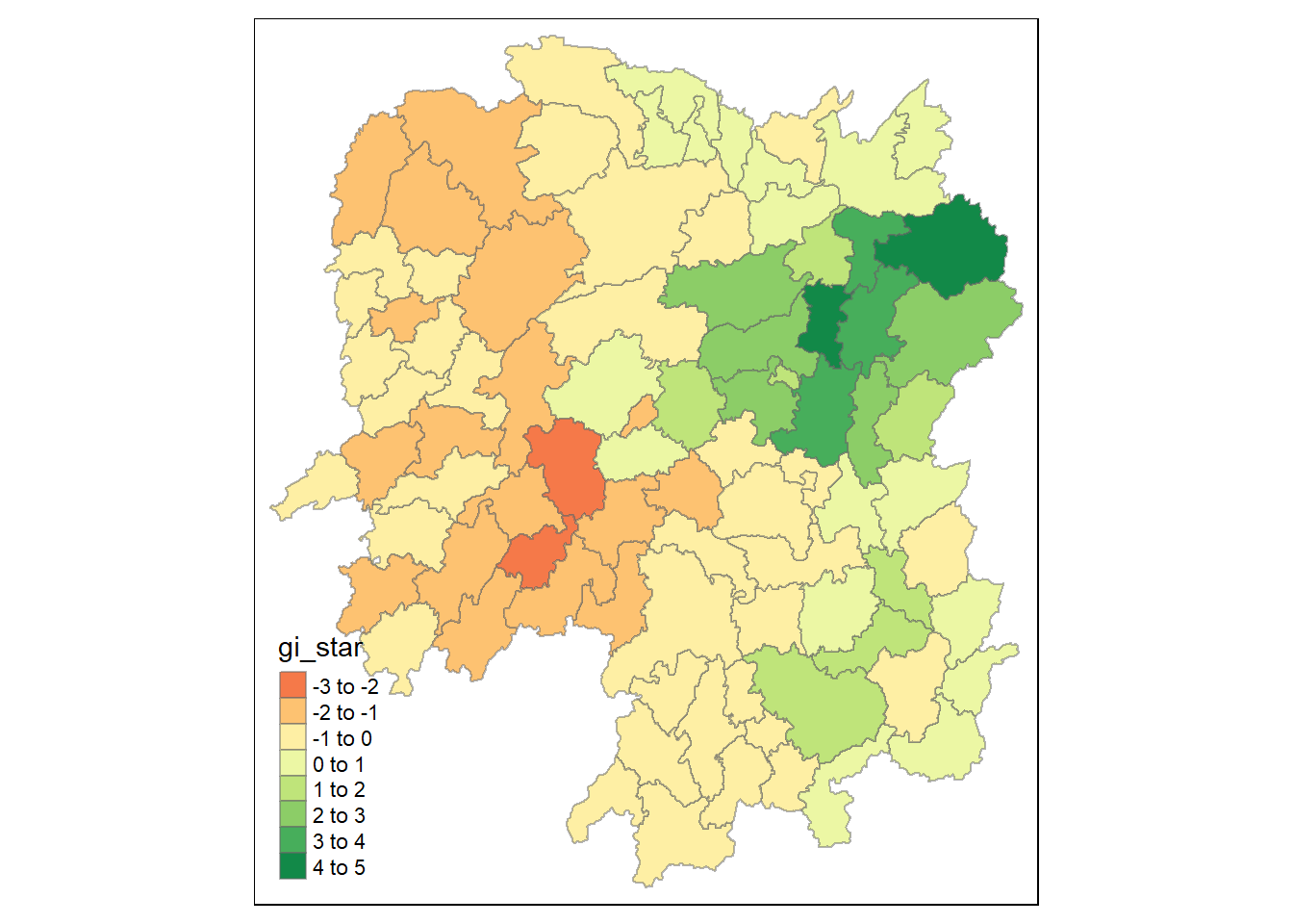
10.2 Visualising p-value of HCSA
In the code chunk below, tmap functions are used to plot the p-values of local Gi* (i.e. p_sim) at the province level.
tmap_mode("plot")
tm_shape(HCSA) +
  tm_fill("p_sim") +
  tm_borders(alpha = 0.5)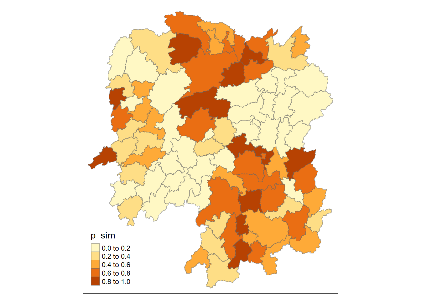
10.3 Visuaising local HCSA
tmap_mode("plot")
map1 <- tm_shape(HCSA) +
  tm_fill("gi_star") +
  tm_borders(alpha = 0.5) +
  tm_view(set.zoom.limits = c(6,8)) +
  tm_layout(main.title = "Gi* of GDPPC",
            main.title.size = 0.8)

map2 <- tm_shape(HCSA) +
  tm_fill("p_value",
          breaks = c(0, 0.001, 0.01, 0.05, 1),
              labels = c("0.001", "0.01", "0.05", "Not sig")) +
  tm_borders(alpha = 0.5) +
  tm_layout(main.title = "p-value of Gi*",
            main.title.size = 0.8)

tmap_arrange(map1, map2, ncol = 2)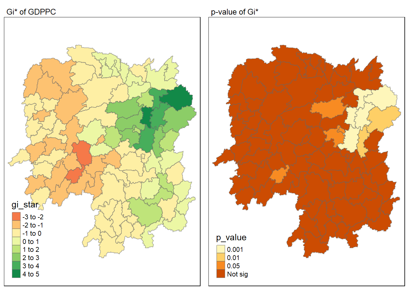
10.4 Visualising hot spot and cold spot areas
HCSA_sig <- HCSA  %>%
  filter(p_sim < 0.05)
tmap_mode("plot")
tm_shape(HCSA) +
  tm_polygons() +
  tm_borders(alpha = 0.5) +
tm_shape(HCSA_sig) +
  tm_fill("cluster") +
  tm_borders(alpha = 0.4)
Note
Figure above reveals that there is one hot spot area and two cold spot areas. Interestingly, the hot spot areas coincide with the High-high cluster identifies by using local Moran’s I method in the earlier sub-section.