pacman::p_load(sf, spdep, GWmodel, SpatialML,
tmap, rsample, Metrics, tidyverse)Hands-on Exercise 8: Geographically Weighted Predictive Models
1. Overview
Predictive modelling uses statistical learning or machine learning techniques to predict outcomes. By and large, the event one wants to predict is in the future. However, a set of known outcome and predictors (also known as variables) will be used to calibrate the predictive models.
Geospatial predictive modelling is conceptually rooted in the principle that the occurrences of events being modeled are limited in distribution. When geographically referenced data are used, occurrences of events are neither uniform nor random in distribution over space. There are geospatial factors (infrastructure, sociocultural, topographic, etc.) that constrain and influence where the locations of events occur. Geospatial predictive modeling attempts to describe those constraints and influences by spatially correlating occurrences of historical geospatial locations with environmental factors that represent those constraints and influences.
1.1 Learning outcome
We will learn how to build predictive model by using geographical random forest method. By the end of this hands-on exercise, you will acquire the skills of:
preparing training and test data sets by using appropriate data sampling methods,
calibrating predictive models by using both geospatial statistical learning and machine learning methods,
comparing and selecting the best model for predicting the future outcome,
predicting the future outcomes by using the best model calibrated.
2. The Data
Aspatial dataset:
- HDB Resale data: a list of HDB resale transacted prices in Singapore from Jan 2017 onwards. It is in csv format which can be downloaded from Data.gov.sg.
Geospatial dataset:
- MP14_SUBZONE_WEB_PL: a polygon feature data providing information of URA 2014 Master Plan Planning Subzone boundary data. It is in ESRI shapefile format. This data set was also downloaded from Data.gov.sg
Locational factors with geographic coordinates:
Downloaded from Data.gov.sg.
Eldercare data is a list of eldercare in Singapore. It is in shapefile format.
Hawker Centre data is a list of hawker centres in Singapore. It is in geojson format.
Parks data is a list of parks in Singapore. It is in geojson format.
Supermarket data is a list of supermarkets in Singapore. It is in geojson format.
CHAS clinics data is a list of CHAS clinics in Singapore. It is in geojson format.
Childcare service data is a list of childcare services in Singapore. It is in geojson format.
Kindergartens data is a list of kindergartens in Singapore. It is in geojson format.
Downloaded from Datamall.lta.gov.sg.
MRT data is a list of MRT/LRT stations in Singapore with the station names and codes. It is in shapefile format.
Bus stops data is a list of bus stops in Singapore. It is in shapefile format.
Locational factors without geographic coordinates:
Downloaded from Data.gov.sg.
- Primary school data is extracted from the list on General information of schools from data.gov portal. It is in csv format.
Retrieved/Scraped from other sources
CBD coordinates obtained from Google.
Shopping malls data is a list of Shopping malls in Singapore obtained from Wikipedia.
Good primary schools is a list of primary schools that are ordered in ranking in terms of popularity and this can be found at Local Salary Forum.
3. Installing and Loading R packages
This code chunk performs 3 tasks:
A list called packages will be created and will consists of all the R packages required to accomplish this exercise.
Check if R packages on package have been installed in R and if not, they will be installed.
After all the R packages have been installed, they will be loaded.
4. Preparing Data
4.1 Reading data file to rds
Reading the input data sets. It is in simple feature data frame.
mdata <- read_rds("data/mdata.rds")4.2 Data Sampling
The entire data are split into training and test data sets with 65% and 35% respectively by using initial_split() of rsample package. rsample is one of the package of tigymodels.
set.seed(1234)
resale_split <- initial_split(mdata,
                              prop = 6.5/10,)
train_data <- training(resale_split)
test_data <- testing(resale_split)write_rds(train_data, "data/train_data.rds")
write_rds(test_data, "data/test_data.rds")5 Computing Correlation Matrix
Before loading the predictors into a predictive model, it is always a good practice to use correlation matrix to examine if there is sign of multicolinearity.
mdata_nogeo <- mdata %>%
  st_drop_geometry()
corrplot::corrplot(cor(mdata_nogeo[, 2:17]),
                   diag = FALSE,
                   order = "AOE",
                   tl.pos = "td",
                   tl.cex = 0.5,
                   method = "number",
                   type = "upper")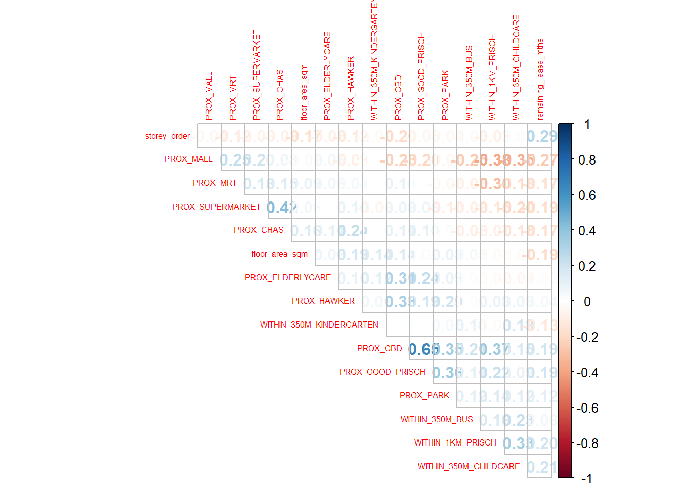
Note
The correlation matrix above shows that all the correlation values are below 0.8. Hence, there is no sign of multicolinearity.
6. Retriving the Stored Data
train_data <- read_rds("data/train_data.rds")
test_data <- read_rds("data/test_data.rds")
7. Building a non-spatial multiple linear regression
price_mlr <- lm(resale_price ~ floor_area_sqm +
                  storey_order + remaining_lease_mths +
                  PROX_CBD + PROX_ELDERLYCARE + PROX_HAWKER +
                  PROX_MRT + PROX_PARK + PROX_MALL +
                  PROX_SUPERMARKET + WITHIN_350M_KINDERGARTEN +
                  WITHIN_350M_CHILDCARE + WITHIN_350M_BUS +
                  WITHIN_1KM_PRISCH,
                data=train_data)
summary(price_mlr)
Call:
lm(formula = resale_price ~ floor_area_sqm + storey_order + remaining_lease_mths +
    PROX_CBD + PROX_ELDERLYCARE + PROX_HAWKER + PROX_MRT + PROX_PARK +
    PROX_MALL + PROX_SUPERMARKET + WITHIN_350M_KINDERGARTEN +
    WITHIN_350M_CHILDCARE + WITHIN_350M_BUS + WITHIN_1KM_PRISCH,
    data = train_data)

Residuals:
    Min      1Q  Median      3Q     Max
-205193  -39120   -1930   36545  472355

Coefficients:
                           Estimate Std. Error t value Pr(>|t|)
(Intercept)              107601.073  10601.261  10.150  < 2e-16 ***
floor_area_sqm             2780.698     90.579  30.699  < 2e-16 ***
storey_order              14299.298    339.115  42.167  < 2e-16 ***
remaining_lease_mths        344.490      4.592  75.027  < 2e-16 ***
PROX_CBD                 -16930.196    201.254 -84.124  < 2e-16 ***
PROX_ELDERLYCARE         -14441.025    994.867 -14.516  < 2e-16 ***
PROX_HAWKER              -19265.648   1273.597 -15.127  < 2e-16 ***
PROX_MRT                 -32564.272   1744.232 -18.670  < 2e-16 ***
PROX_PARK                 -5712.625   1483.885  -3.850 0.000119 ***
PROX_MALL                -14717.388   2007.818  -7.330 2.47e-13 ***
PROX_SUPERMARKET         -26881.938   4189.624  -6.416 1.46e-10 ***
WITHIN_350M_KINDERGARTEN   8520.472    632.812  13.464  < 2e-16 ***
WITHIN_350M_CHILDCARE     -4510.650    354.015 -12.741  < 2e-16 ***
WITHIN_350M_BUS             813.493    222.574   3.655 0.000259 ***
WITHIN_1KM_PRISCH         -8010.834    491.512 -16.298  < 2e-16 ***
---
Signif. codes:  0 '***' 0.001 '**' 0.01 '*' 0.05 '.' 0.1 ' ' 1

Residual standard error: 61650 on 10320 degrees of freedom
Multiple R-squared:  0.7373,    Adjusted R-squared:  0.737
F-statistic: 2069 on 14 and 10320 DF, p-value: < 2.2e-16write_rds(price_mlr, "data/price_mlr.rds" ) 8. gwr predictive method
In this section, you will learn how to calibrate a model to predict HDB resale price by using geographically weighted regression method of GWmodel package.
8.1 Converting the sf data.frame to SpatialPointDataFrame
train_data_sp <- as_Spatial(train_data)
train_data_sp
class : SpatialPointsDataFrame
features : 10335
extent : 11597.31, 42623.63, 28217.39, 48741.06 (xmin, xmax, ymin, ymax)
crs : +proj=tmerc +lat_0=1.36666666666667 +lon_0=103.833333333333 +k=1 +x_0=28001.642 +y_0=38744.572 +ellps=WGS84 +towgs84=0,0,0,0,0,0,0 +units=m +no_defs
variables : 17
names : resale_price, floor_area_sqm, storey_order, remaining_lease_mths, PROX_CBD, PROX_ELDERLYCARE, PROX_HAWKER, PROX_MRT, PROX_PARK, PROX_GOOD_PRISCH, PROX_MALL, PROX_CHAS, PROX_SUPERMARKET, WITHIN_350M_KINDERGARTEN, WITHIN_350M_CHILDCARE, ...
min values : 218000, 74, 1, 555, 0.999393538715878, 1.98943787433087e-08, 0.0333358643817954, 0.0220407324774434, 0.0441643212802781, 0.0652540365486641, 0, 6.20621206270077e-09, 1.21715176356525e-07, 0, 0, ...
max values : 1186888, 133, 17, 1164, 19.6500691667807, 3.30163731686804, 2.86763031236184, 2.13060636038504, 2.41313695915468, 10.6223726149914, 2.27100643784442, 0.808332738794272, 1.57131703651196, 7, 20, ... 8.2 Computing adaptive bandwidth
Next, bw.gwr() of GWmodel package will be used to determine the optimal bandwidth to be used.
Note
The code chunk below is used to determine adaptive bandwidth and CV method is used to determine the optimal bandwidth.
bw_adaptive <- bw.gwr(resale_price ~ floor_area_sqm +
                  storey_order + remaining_lease_mths +
                  PROX_CBD + PROX_ELDERLYCARE + PROX_HAWKER +
                  PROX_MRT + PROX_PARK + PROX_MALL +
                  PROX_SUPERMARKET + WITHIN_350M_KINDERGARTEN +
                  WITHIN_350M_CHILDCARE + WITHIN_350M_BUS +
                  WITHIN_1KM_PRISCH,
                  data=train_data_sp,
                  approach="CV",
                  kernel="gaussian",
                  adaptive=TRUE,
                  longlat=FALSE)
Take a cup of tea and have a break, it will take a few minutes.
-----A kind suggestion from GWmodel development group
Adaptive bandwidth: 6395 CV score: 3.60536e+13
Adaptive bandwidth: 3960 CV score: 3.320316e+13
Adaptive bandwidth: 2455 CV score: 2.928339e+13
Adaptive bandwidth: 1524 CV score: 2.550957e+13
Adaptive bandwidth: 950 CV score: 1.95632e+13
Adaptive bandwidth: 593 CV score: 1.58347e+13
Adaptive bandwidth: 375 CV score: 1.310042e+13
Adaptive bandwidth: 237 CV score: 1.113152e+13
Adaptive bandwidth: 155 CV score: 9.572037e+12
Adaptive bandwidth: 101 CV score: 8.457003e+12
Adaptive bandwidth: 71 CV score: 7.605058e+12
Adaptive bandwidth: 49 CV score: 6.965752e+12
Adaptive bandwidth: 38 CV score: 8.249935e+12
Adaptive bandwidth: 58 CV score: 7.275234e+12
Adaptive bandwidth: 45 CV score: 6.871439e+12
Adaptive bandwidth: 41 CV score: 6.7928e+12
Adaptive bandwidth: 40 CV score: 6.780447e+12
Adaptive bandwidth: 38 CV score: 8.249935e+12
Adaptive bandwidth: 40 CV score: 6.780447e+12 The result shows that 40 neighbour points will be the optimal bandwidth to be used if adaptive bandwidth is used for this data set.
write_rds(bw_adaptive, "data/bw_adaptive.rds")8.3 Constructing the adaptive bandwidth gwr model
First, let us call the save bandwidth by using the code chunk below.
bw_adaptive <- read_rds("data/bw_adaptive.rds")Now, we can go ahead to calibrate the gwr-based hedonic pricing model by using adaptive bandwidth and Gaussian kernel as shown in the code chunk below.
gwr_adaptive <- gwr.basic(formula = resale_price ~
                            floor_area_sqm + storey_order +
                            remaining_lease_mths + PROX_CBD +
                            PROX_ELDERLYCARE + PROX_HAWKER +
                            PROX_MRT + PROX_PARK + PROX_MALL +
                            PROX_SUPERMARKET + WITHIN_350M_KINDERGARTEN +
                            WITHIN_350M_CHILDCARE + WITHIN_350M_BUS +
                            WITHIN_1KM_PRISCH,
                          data=train_data_sp,
                          bw=bw_adaptive,
                          kernel = 'gaussian',
                          adaptive=TRUE,
                          longlat = FALSE)
The code chunk below will be used to save the model in rds format for future use.
write_rds(gwr_adaptive, "data/gwr_adaptive.rds")8.4 Retrieve gwr output object
gwr_adaptive <- read_rds("data/gwr_adaptive.rds")The code below can be used to display the model output.
gwr_adaptive ***********************************************************************
* Package GWmodel *
***********************************************************************
Program starts at: 2024-10-21 00:08:39.754313
Call:
gwr.basic(formula = resale_price ~ floor_area_sqm + storey_order +
remaining_lease_mths + PROX_CBD + PROX_ELDERLYCARE + PROX_HAWKER +
PROX_MRT + PROX_PARK + PROX_MALL + PROX_SUPERMARKET + WITHIN_350M_KINDERGARTEN +
WITHIN_350M_CHILDCARE + WITHIN_350M_BUS + WITHIN_1KM_PRISCH,
data = train_data_sp, bw = bw_adaptive, kernel = "gaussian",
adaptive = TRUE, longlat = FALSE)
Dependent (y) variable: resale_price
Independent variables: floor_area_sqm storey_order remaining_lease_mths PROX_CBD PROX_ELDERLYCARE PROX_HAWKER PROX_MRT PROX_PARK PROX_MALL PROX_SUPERMARKET WITHIN_350M_KINDERGARTEN WITHIN_350M_CHILDCARE WITHIN_350M_BUS WITHIN_1KM_PRISCH
Number of data points: 10335
***********************************************************************
* Results of Global Regression *
***********************************************************************
Call:
lm(formula = formula, data = data)
Residuals:
Min 1Q Median 3Q Max
-205193 -39120 -1930 36545 472355
Coefficients:
Estimate Std. Error t value Pr(>|t|)
(Intercept) 107601.073 10601.261 10.150 < 2e-16 ***
floor_area_sqm 2780.698 90.579 30.699 < 2e-16 ***
storey_order 14299.298 339.115 42.167 < 2e-16 ***
remaining_lease_mths 344.490 4.592 75.027 < 2e-16 ***
PROX_CBD -16930.196 201.254 -84.124 < 2e-16 ***
PROX_ELDERLYCARE -14441.025 994.867 -14.516 < 2e-16 ***
PROX_HAWKER -19265.648 1273.597 -15.127 < 2e-16 ***
PROX_MRT -32564.272 1744.232 -18.670 < 2e-16 ***
PROX_PARK -5712.625 1483.885 -3.850 0.000119 ***
PROX_MALL -14717.388 2007.818 -7.330 2.47e-13 ***
PROX_SUPERMARKET -26881.938 4189.624 -6.416 1.46e-10 ***
WITHIN_350M_KINDERGARTEN 8520.472 632.812 13.464 < 2e-16 ***
WITHIN_350M_CHILDCARE -4510.650 354.015 -12.741 < 2e-16 ***
WITHIN_350M_BUS 813.493 222.574 3.655 0.000259 ***
WITHIN_1KM_PRISCH -8010.834 491.512 -16.298 < 2e-16 ***
---Significance stars
Signif. codes: 0 '***' 0.001 '**' 0.01 '*' 0.05 '.' 0.1 ' ' 1
Residual standard error: 61650 on 10320 degrees of freedom
Multiple R-squared: 0.7373
Adjusted R-squared: 0.737
F-statistic: 2069 on 14 and 10320 DF, p-value: < 2.2e-16
***Extra Diagnostic information
Residual sum of squares: 3.922202e+13
Sigma(hat): 61610.08
AIC: 257320.2
AICc: 257320.3
BIC: 247249
***********************************************************************
* Results of Geographically Weighted Regression *
***********************************************************************
*********************Model calibration information*********************
Kernel function: gaussian
Adaptive bandwidth: 40 (number of nearest neighbours)
Regression points: the same locations as observations are used.
Distance metric: Euclidean distance metric is used.
****************Summary of GWR coefficient estimates:******************
Min. 1st Qu. Median 3rd Qu.
Intercept -3.2478e+08 -4.7727e+05 -8.3004e+03 5.5025e+05
floor_area_sqm -2.8714e+04 1.4475e+03 2.3011e+03 3.3900e+03
storey_order 3.3186e+03 8.5899e+03 1.0826e+04 1.3397e+04
remaining_lease_mths -1.4431e+03 2.6063e+02 3.9048e+02 5.2865e+02
PROX_CBD -1.0837e+07 -5.7697e+04 -1.3787e+04 2.6552e+04
PROX_ELDERLYCARE -3.2195e+07 -4.0643e+04 1.0562e+04 6.1054e+04
PROX_HAWKER -2.3985e+08 -5.1365e+04 3.0026e+03 6.4287e+04
PROX_MRT -1.1632e+07 -1.0488e+05 -4.9373e+04 5.1037e+03
PROX_PARK -6.5961e+06 -4.8671e+04 -8.8128e+02 5.3498e+04
PROX_MALL -1.8112e+07 -7.4238e+04 -1.3982e+04 4.9779e+04
PROX_SUPERMARKET -4.5761e+06 -6.3461e+04 -1.7429e+04 3.5616e+04
WITHIN_350M_KINDERGARTEN -4.1823e+05 -6.0040e+03 9.0209e+01 4.7127e+03
WITHIN_350M_CHILDCARE -1.0273e+05 -2.2375e+03 2.6668e+02 2.6388e+03
WITHIN_350M_BUS -1.1757e+05 -1.4719e+03 1.1626e+02 1.7584e+03
WITHIN_1KM_PRISCH -6.6465e+05 -5.5959e+03 2.6916e+02 5.7500e+03
Max.
Intercept 1.6493e+08
floor_area_sqm 5.0907e+04
storey_order 2.9537e+04
remaining_lease_mths 1.8119e+03
PROX_CBD 2.2411e+07
PROX_ELDERLYCARE 8.2444e+07
PROX_HAWKER 5.9654e+06
PROX_MRT 2.0189e+08
PROX_PARK 1.5188e+07
PROX_MALL 1.0443e+07
PROX_SUPERMARKET 3.8330e+06
WITHIN_350M_KINDERGARTEN 6.6799e+05
WITHIN_350M_CHILDCARE 1.0802e+05
WITHIN_350M_BUS 3.7313e+04
WITHIN_1KM_PRISCH 5.0231e+05
************************Diagnostic information*************************
Number of data points: 10335
Effective number of parameters (2trace(S) - trace(S'S)): 1730.101
Effective degrees of freedom (n-2trace(S) + trace(S'S)): 8604.899
AICc (GWR book, Fotheringham, et al. 2002, p. 61, eq 2.33): 238871.9
AIC (GWR book, Fotheringham, et al. 2002,GWR p. 96, eq. 4.22): 237036.9
BIC (GWR book, Fotheringham, et al. 2002,GWR p. 61, eq. 2.34): 238209.1
Residual sum of squares: 4.829191e+12
R-square value: 0.967657
Adjusted R-square value: 0.9611534
***********************************************************************
Program stops at: 2024-10-21 00:10:01.642013 8.5 Converting the test data from sf data.frame to SpatialPointDataFrame
test_data_sp <- test_data %>%
  as_Spatial()
test_data_sp
class : SpatialPointsDataFrame
features : 5566
extent : 11597.31, 42623.63, 28287.8, 48669.59 (xmin, xmax, ymin, ymax)
crs : +proj=tmerc +lat_0=1.36666666666667 +lon_0=103.833333333333 +k=1 +x_0=28001.642 +y_0=38744.572 +ellps=WGS84 +towgs84=0,0,0,0,0,0,0 +units=m +no_defs
variables : 17
names : resale_price, floor_area_sqm, storey_order, remaining_lease_mths, PROX_CBD, PROX_ELDERLYCARE, PROX_HAWKER, PROX_MRT, PROX_PARK, PROX_GOOD_PRISCH, PROX_MALL, PROX_CHAS, PROX_SUPERMARKET, WITHIN_350M_KINDERGARTEN, WITHIN_350M_CHILDCARE, ...
min values : 230888, 74, 1, 546, 1.00583660772922, 3.34897933104965e-07, 0.0474019664161957, 0.0414043955932523, 0.0502664084494264, 0.0907500295577619, 0, 4.55547870890763e-09, 1.21715176356525e-07, 0, 0, ...
max values : 1050000, 138, 14, 1151, 19.632402730488, 3.30163731686804, 2.83106651960209, 2.13060636038504, 2.41313695915468, 10.6169590126272, 2.26056404492346, 0.79249074802552, 1.53786629004208, 7, 16, ... 8.6 Computing adaptive bandwidth for the test data
gwr_bw_test_adaptive <- bw.gwr(resale_price ~ floor_area_sqm +
                  storey_order + remaining_lease_mths +
                  PROX_CBD + PROX_ELDERLYCARE + PROX_HAWKER +
                  PROX_MRT + PROX_PARK + PROX_MALL +
                  PROX_SUPERMARKET + WITHIN_350M_KINDERGARTEN +
                  WITHIN_350M_CHILDCARE + WITHIN_350M_BUS +
                  WITHIN_1KM_PRISCH,
                  data=test_data_sp,
                  approach="CV",
                  kernel="gaussian",
                  adaptive=TRUE,
                  longlat=FALSE)
Take a cup of tea and have a break, it will take a few minutes.
-----A kind suggestion from GWmodel development group
Adaptive bandwidth: 3447 CV score: 1.902155e+13
Adaptive bandwidth: 2138 CV score: 1.752645e+13
Adaptive bandwidth: 1328 CV score: 1.556299e+13
Adaptive bandwidth: 828 CV score: 1.357498e+13
Adaptive bandwidth: 518 CV score: 1.030751e+13
Adaptive bandwidth: 327 CV score: 8.348364e+12
Adaptive bandwidth: 208 CV score: 6.860544e+12
Adaptive bandwidth: 135 CV score: 5.969504e+12
Adaptive bandwidth: 89 CV score: 5.242221e+12
Adaptive bandwidth: 62 CV score: 4.742767e+12
Adaptive bandwidth: 43 CV score: 4.357839e+12
Adaptive bandwidth: 34 CV score: 4.125848e+12
Adaptive bandwidth: 25 CV score: 4.04299e+12
Adaptive bandwidth: 23 CV score: 1.549626e+13
Adaptive bandwidth: 30 CV score: 4.074906e+12
Adaptive bandwidth: 25 CV score: 4.04299e+12 8.7 Computing predicted values of the test data
8.7.1 Inspect the Spatial Coordinates
We need to confirm that your train_data_sp and test_data_sp objects have valid, non-empty spatial coordinates. We can check the coordinates using the below code chunk.
head(coordinates(train_data_sp)) coords.x1 coords.x2
[1,] 39421.99 37094.13
[2,] 36395.05 31714.45
[3,] 41466.54 38691.58
[4,] 35027.93 43052.26
[5,] 27363.82 48032.56
[6,] 28871.91 46265.93head(coordinates(test_data_sp)) coords.x1 coords.x2
[1,] 28423.42 39745.94
[2,] 30550.38 39588.77
[3,] 28240.06 39477.60
[4,] 30637.92 39516.90
[5,] 30347.48 38995.85
[6,] 28325.75 39700.70This will help us see if there are actual coordinate points in the data.
8.7.2 Check for Overlapping Points
One common issue is that some points in your test_data_sp may not have corresponding points close enough in train_data_sp to perform GWR. This can happen if the test data points are outside the area covered by the training data.
We can check if test_data_sp points fall within the spatial extent of train_data_sp using the below code chunk.
bbox(train_data_sp) min max
coords.x1 11597.31 42623.63
coords.x2 28217.39 48741.06bbox(test_data_sp) min max
coords.x1 11597.31 42623.63
coords.x2 28287.80 48669.59Make sure the bounding boxes (extents) of your training and test data overlap.
8.7.3 Check if the Data is Too Sparse
If the data is very sparse or scattered, the selected bandwidth (bw=40) may be too small to cover any points for some locations. In such a case, we could:
Increase the bandwidth to cover more points.
Use an adaptive bandwidth (
adaptive=TRUE) with a larger range. This adapts the bandwidth to ensure each regression point has enough neighbors.
8.7.4 Test a Small Sample
We could try using a smaller subset of your data (both train_data_sp and test_data_sp) to see if the issue is caused by a particular part of your dataset. We can randomly sample a few points for testing.
train_sample <- train_data_sp[sample(1:nrow(train_data_sp), 100), ]
test_sample <- test_data_sp[sample(1:nrow(test_data_sp), 50), ]
gwr_pred <- gwr.predict(formula = resale_price ~
floor_area_sqm + storey_order +
remaining_lease_mths + PROX_CBD +
PROX_ELDERLYCARE + PROX_HAWKER +
PROX_MRT + PROX_PARK + PROX_MALL +
PROX_SUPERMARKET + WITHIN_350M_KINDERGARTEN +
WITHIN_350M_CHILDCARE + WITHIN_350M_BUS +
WITHIN_1KM_PRISCH,
data=train_sample,
predictdata = test_sample,
bw=40,
kernel = 'gaussian',
adaptive=TRUE,
longlat = FALSE)9. Preparing coordinates data
9.1 Extracting coordinates data
The code chunk below extract the x,y coordinates of the full, training and test data sets.
coords <- st_coordinates(mdata)
coords_train <- st_coordinates(train_data)
coords_test <- st_coordinates(test_data)
Before continue, we write all the output into rds for future used.
coords_train <- write_rds(coords_train, "data/coords_train.rds" )
coords_test <- write_rds(coords_test, "data/coords_test.rds" )
9.2 Droping geometry field
First, we will drop geometry column of the sf data.frame by using st_drop_geometry() of sf package.
train_data <- train_data %>%
  st_drop_geometry()
10. Calibrating Random Forest Model
In this section, you will learn how to calibrate a model to predict HDB resale price by using random forest function of ranger package.
set.seed(1234)
rf <- ranger(resale_price ~ floor_area_sqm + storey_order +
               remaining_lease_mths + PROX_CBD + PROX_ELDERLYCARE +
               PROX_HAWKER + PROX_MRT + PROX_PARK + PROX_MALL +
               PROX_SUPERMARKET + WITHIN_350M_KINDERGARTEN +
               WITHIN_350M_CHILDCARE + WITHIN_350M_BUS +
               WITHIN_1KM_PRISCH,
             data=train_data)
rf
Ranger result
Call:
ranger(resale_price ~ floor_area_sqm + storey_order + remaining_lease_mths + PROX_CBD + PROX_ELDERLYCARE + PROX_HAWKER + PROX_MRT + PROX_PARK + PROX_MALL + PROX_SUPERMARKET + WITHIN_350M_KINDERGARTEN + WITHIN_350M_CHILDCARE + WITHIN_350M_BUS + WITHIN_1KM_PRISCH, data = train_data)
Type: Regression
Number of trees: 500
Sample size: 10335
Number of independent variables: 14
Mtry: 3
Target node size: 5
Variable importance mode: none
Splitrule: variance
OOB prediction error (MSE): 728602496
R squared (OOB): 0.9495728 write_rds(rf, "data/rf.rds")rf <- read_rds("data/rf.rds")
rfRanger result
Call:
ranger(resale_price ~ floor_area_sqm + storey_order + remaining_lease_mths + PROX_CBD + PROX_ELDERLYCARE + PROX_HAWKER + PROX_MRT + PROX_PARK + PROX_MALL + PROX_SUPERMARKET + WITHIN_350M_KINDERGARTEN + WITHIN_350M_CHILDCARE + WITHIN_350M_BUS + WITHIN_1KM_PRISCH, data = train_data)
Type: Regression
Number of trees: 500
Sample size: 10335
Number of independent variables: 14
Mtry: 3
Target node size: 5
Variable importance mode: none
Splitrule: variance
OOB prediction error (MSE): 728602496
R squared (OOB): 0.9495728 11. Calibrating Geographical Random Forest Model
In this section, you will learn how to calibrate a model to predict HDB resale price by using grf() of SpatialML package.
11.1 Calibrating using training data
The code chunk below calibrate a geographic ranform forest model by using grf() of SpatialML package.
set.seed(1234)

train_sample <- train_data[sample(1:nrow(train_data), 100), ]  # Select 100 random rows
coords_sample <- coords_train[sample(1:nrow(coords_train), 100), ]

gwRF_adaptive <- grf(formula = resale_price ~ floor_area_sqm + storey_order +
                              remaining_lease_mths + PROX_CBD + PROX_ELDERLYCARE +
                              PROX_HAWKER + PROX_MRT + PROX_PARK + PROX_MALL +
                              PROX_SUPERMARKET + WITHIN_350M_KINDERGARTEN +
                              WITHIN_350M_CHILDCARE + WITHIN_350M_BUS +
                              WITHIN_1KM_PRISCH,
                            dframe = train_sample,
                            bw = 55,
                            kernel = "adaptive",
                            coords = coords_sample)
Ranger result
Call:
ranger(resale_price ~ floor_area_sqm + storey_order + remaining_lease_mths + PROX_CBD + PROX_ELDERLYCARE + PROX_HAWKER + PROX_MRT + PROX_PARK + PROX_MALL + PROX_SUPERMARKET + WITHIN_350M_KINDERGARTEN + WITHIN_350M_CHILDCARE + WITHIN_350M_BUS + WITHIN_1KM_PRISCH, data = train_sample, num.trees = 500, mtry = 4, importance = "impurity", num.threads = NULL)
Type: Regression
Number of trees: 500
Sample size: 100
Number of independent variables: 14
Mtry: 4
Target node size: 5
Variable importance mode: impurity
Splitrule: variance
OOB prediction error (MSE): 5117322740
R squared (OOB): 0.5755322
floor_area_sqm storey_order remaining_lease_mths
73623908352 112564545878 193798920761
PROX_CBD PROX_ELDERLYCARE PROX_HAWKER
329190514912 126433351861 39908320280
PROX_MRT PROX_PARK PROX_MALL
42929532875 44689246051 38006750535
PROX_SUPERMARKET WITHIN_350M_KINDERGARTEN WITHIN_350M_CHILDCARE
48269369872 11262414493 21472348287
WITHIN_350M_BUS WITHIN_1KM_PRISCH
29833749925 21678554121
Min. 1st Qu. Median Mean 3rd Qu. Max.
-189841 -63195 -23035 -2356 44440 379786
Min. 1st Qu. Median Mean 3rd Qu. Max.
-30325.7 -7565.5 -2092.7 195.5 6405.0 61607.3
Min Max Mean StD
floor_area_sqm 8907048410 96411360080 33176223893 25087408764
storey_order 11505368822 219510158197 64939881876 70730929998
remaining_lease_mths 15136295713 239825073747 90571950227 78264722831
PROX_CBD 70366740612 261668577980 149022125762 56418220920
PROX_ELDERLYCARE 34654119694 128263862589 65856466959 25391719050
PROX_HAWKER 14869195104 71395165481 39916329777 15933256621
PROX_MRT 10771637537 67817159573 27385395195 17259064961
PROX_PARK 9643476972 77520338798 33693368304 15507900524
PROX_MALL 9750435785 53908526850 25545868981 8769947166
PROX_SUPERMARKET 18333010935 52013994587 30042093157 8325340144
WITHIN_350M_KINDERGARTEN 2364872571 43471919780 10713251108 9122261123
WITHIN_350M_CHILDCARE 6036843938 34196426417 14310495138 8430267554
WITHIN_350M_BUS 10133623617 35951454792 19544963213 6010940660
WITHIN_1KM_PRISCH 6774039313 45136073952 21724141890 11846915978Let’s save the model output by using the code chunk below.
write_rds(gwRF_adaptive, "data/gwRF_adaptive.rds")The code chunk below can be used to retrieve the save model in future.
gwRF_adaptive <- read_rds("data/gwRF_adaptive.rds")11.2 Predicting by using test data
11.2.1 Preparing the test data
The code chunk below will be used to combine the test data with its corresponding coordinates data.
test_data <- cbind(test_data, coords_test) %>%
  st_drop_geometry()
11.2.2 Predicting with test data
Next, predict.grf() of spatialML package will be used to predict the resale value by using the test data and gwRF_adaptive model calibrated earlier.
gwRF_pred <- predict.grf(gwRF_adaptive,
                           test_data,
                           x.var.name="X",
                           y.var.name="Y",
                           local.w=1,
                           global.w=0)
Before moving on, let us save the output into rds file for future use.
GRF_pred <- write_rds(gwRF_pred, "data/GRF_pred.rds")11.2.3 Converting the predicting output into a data frame
The output of the predict.grf() is a vector of predicted values. It is wiser to convert it into a data frame for further visualisation and analysis.
GRF_pred <- read_rds("data/GRF_pred.rds")
GRF_pred_df <- as.data.frame(GRF_pred)
In the code chunk below, cbind() is used to append the predicted values onto test_datathe
test_data_p <- cbind(test_data, GRF_pred_df)write_rds(test_data_p, "data/test_data_p.rds")11.3 Calculating Root Mean Square Error
The root mean square error (RMSE) allows us to measure how far predicted values are from observed values in a regression analysis. In the code chunk below, rmse() of Metrics package is used to compute the RMSE.
rmse(test_data_p$resale_price,
     test_data_p$GRF_pred)
[1] 93600.1511.4 Visualising the predicted values
Alternatively, scatterplot can be used to visualise the actual resale price and the predicted resale price by using the code chunk below.
ggplot(data = test_data_p,
       aes(x = GRF_pred,
           y = resale_price)) +
  geom_point()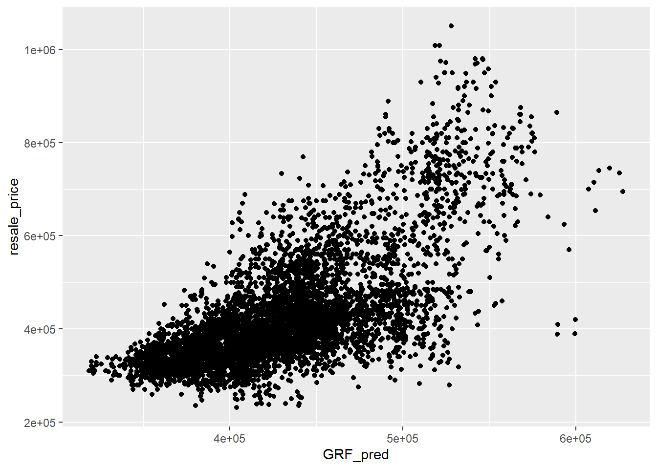
Note
A better predictive model should have the scatter point close to the diagonal line. The scatter plot can be also used to detect if any outliers in the model.