pacman::p_load(sf, spdep, GWmodel, SpatialML,
               tmap, rsample, Metrics, tidyverse,
knitr, kableExtra)In-class Exercise 8: Supplement to Hands-on Exercise 8
1. Getting Started
1.1 Installing and Loading R packages
2. Preparing Data
mdata <- read_rds("data/mdata.rds")Calibrating predictive models are computational intensive, especially random forest method is used. For quick prototyping, a 10% sample will be selected at random from the data by using the code chunk below.
set.seed(1234)
HDB_sample <- mdata %>%
  sample_n(1500)
Warning
When using GWmodel to calibrate explanatory or predictive models, it is very important to ensure that there are no overlapping point features
The code chunk below is used to check if there are overlapping point features.
overlapping_points <- HDB_sample %>%
  mutate(overlap = lengths(st_equals(., .)) > 1)
In the code code chunk below, st_jitter() of sf package is used to move the point features by 5m to avoid overlapping point features.
HDB_sample <- HDB_sample %>%
  st_jitter(amount = 5)
3. Data Sampling
The entire data are split into training and test data sets with 65% and 35% respectively by using initial_split() of rsample package. rsample is one of the package of tigymodels.
set.seed(1234)
resale_split <- initial_split(HDB_sample,
                              prop = 6.67/10,)
train_data <- training(resale_split)
test_data <- testing(resale_split)
4. Multicollinearity check
In order to avoid multicollineariy. In the code chunk below, ggcorrmat() of ggstatsplot is used to plot a correlation matrix to check if there are pairs of highly correlated independent variables.
mdata_nogeo <- mdata %>%
  st_drop_geometry()
ggstatsplot::ggcorrmat(mdata_nogeo[, 2:17])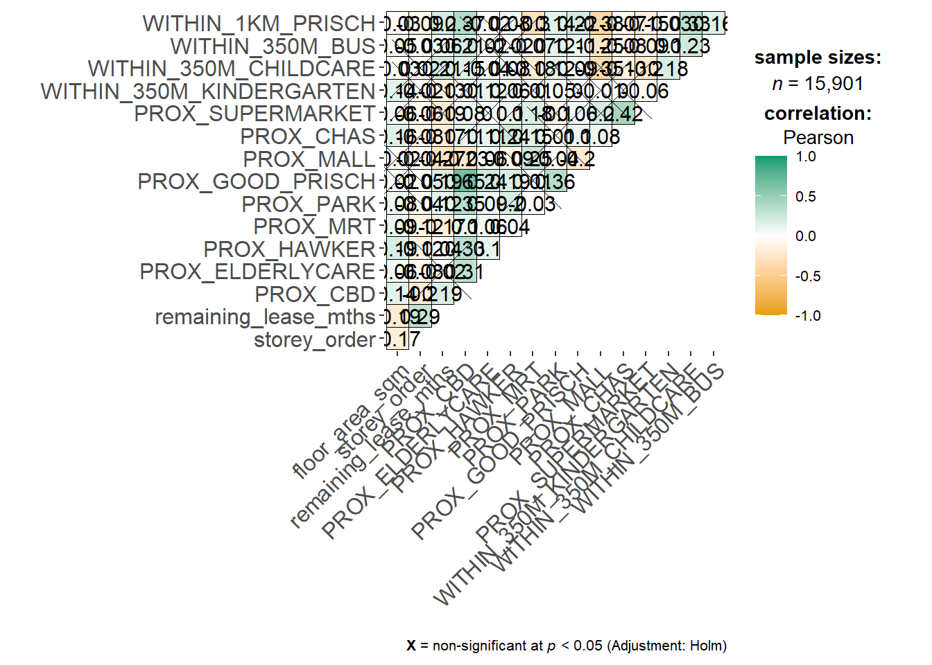
5. Building a non-spatial multiple linear regression
price_mlr <- lm(resale_price ~ floor_area_sqm +
                  storey_order + remaining_lease_mths +
                  PROX_CBD + PROX_ELDERLYCARE + PROX_HAWKER +
                  PROX_MRT + PROX_PARK + PROX_MALL +
                  PROX_SUPERMARKET + WITHIN_350M_KINDERGARTEN +
                  WITHIN_350M_CHILDCARE + WITHIN_350M_BUS +
                  WITHIN_1KM_PRISCH,
                data=train_data)
olsrr::ols_regress(price_mlr)
Model Summary
--------------------------------------------------------------------------
R 0.862 RMSE 60813.316
R-Squared 0.742 MSE 3754578098.252
Adj. R-Squared 0.739 Coef. Var 14.255
Pred R-Squared 0.734 AIC 24901.005
MAE 45987.256 SBC 24979.529
--------------------------------------------------------------------------
RMSE: Root Mean Square Error
MSE: Mean Square Error
MAE: Mean Absolute Error
AIC: Akaike Information Criteria
SBC: Schwarz Bayesian Criteria
ANOVA
-------------------------------------------------------------------------------
Sum of
Squares DF Mean Square F Sig.
-------------------------------------------------------------------------------
Regression 1.065708e+13 14 761220078101.236 202.745 0.0000
Residual 3.698259e+12 985 3754578098.252
Total 1.435534e+13 999
-------------------------------------------------------------------------------
Parameter Estimates
------------------------------------------------------------------------------------------------------------------
model Beta Std. Error Std. Beta t Sig lower upper
------------------------------------------------------------------------------------------------------------------
(Intercept) 115703.696 34303.409 3.373 0.001 48387.533 183019.860
floor_area_sqm 2778.618 292.262 0.165 9.507 0.000 2205.089 3352.146
storey_order 12698.165 1070.950 0.211 11.857 0.000 10596.559 14799.771
remaining_lease_mths 350.252 14.596 0.450 23.997 0.000 321.610 378.894
PROX_CBD -16225.588 630.092 -0.572 -25.751 0.000 -17462.065 -14989.110
PROX_ELDERLYCARE -11330.930 3220.845 -0.061 -3.518 0.000 -17651.436 -5010.423
PROX_HAWKER -19964.070 4021.046 -0.087 -4.965 0.000 -27854.872 -12073.268
PROX_MRT -39652.516 5412.288 -0.130 -7.326 0.000 -50273.456 -29031.577
PROX_PARK -15878.322 4609.199 -0.061 -3.445 0.001 -24923.300 -6833.344
PROX_MALL -15910.922 6438.111 -0.048 -2.471 0.014 -28544.911 -3276.933
PROX_SUPERMARKET -18928.514 13304.965 -0.025 -1.423 0.155 -45037.848 7180.821
WITHIN_350M_KINDERGARTEN 9309.735 2024.293 0.079 4.599 0.000 5337.313 13282.157
WITHIN_350M_CHILDCARE -1619.514 1180.948 -0.026 -1.371 0.171 -3936.977 697.948
WITHIN_350M_BUS -447.695 738.715 -0.011 -0.606 0.545 -1897.331 1001.940
WITHIN_1KM_PRISCH -10698.012 1543.511 -0.138 -6.931 0.000 -13726.960 -7669.065
------------------------------------------------------------------------------------------------------------------6. Multicollinearity check with VIF
6.1 VIF
vif <- performance::check_collinearity(price_mlr)
kable(vif,
      caption = "Variance Inflation Factor (VIF) Results") %>%
kable_styling(font_size = 18) | Term | VIF | VIF_CI_low | VIF_CI_high | SE_factor | Tolerance | Tolerance_CI_low | Tolerance_CI_high |
|---|---|---|---|---|---|---|---|
| floor_area_sqm | 1.146686 | 1.085743 | 1.250945 | 1.070834 | 0.8720785 | 0.7993954 | 0.9210287 |
| storey_order | 1.206020 | 1.135720 | 1.312734 | 1.098189 | 0.8291736 | 0.7617690 | 0.8804986 |
| remaining_lease_mths | 1.343645 | 1.254833 | 1.463410 | 1.159157 | 0.7442440 | 0.6833358 | 0.7969186 |
| PROX_CBD | 1.887898 | 1.733977 | 2.074096 | 1.374008 | 0.5296898 | 0.4821378 | 0.5767088 |
| PROX_ELDERLYCARE | 1.140418 | 1.080572 | 1.244716 | 1.067904 | 0.8768712 | 0.8033960 | 0.9254357 |
| PROX_HAWKER | 1.183865 | 1.116887 | 1.289223 | 1.088056 | 0.8446907 | 0.7756609 | 0.8953457 |
| PROX_MRT | 1.211390 | 1.140307 | 1.318485 | 1.100632 | 0.8254980 | 0.7584464 | 0.8769566 |
| PROX_PARK | 1.186122 | 1.118797 | 1.291599 | 1.089092 | 0.8430839 | 0.7742340 | 0.8938169 |
| PROX_MALL | 1.435504 | 1.335252 | 1.565736 | 1.198125 | 0.6966193 | 0.6386771 | 0.7489224 |
| PROX_SUPERMARKET | 1.226727 | 1.153448 | 1.335000 | 1.107577 | 0.8151773 | 0.7490638 | 0.8669656 |
| WITHIN_350M_KINDERGARTEN | 1.123989 | 1.067172 | 1.228865 | 1.060183 | 0.8896886 | 0.8137594 | 0.9370564 |
| WITHIN_350M_CHILDCARE | 1.387119 | 1.292841 | 1.511748 | 1.177760 | 0.7209189 | 0.6614860 | 0.7734902 |
| WITHIN_350M_BUS | 1.193498 | 1.125056 | 1.299398 | 1.092473 | 0.8378731 | 0.7695869 | 0.8888447 |
| WITHIN_1KM_PRISCH | 1.508943 | 1.399770 | 1.647930 | 1.228390 | 0.6627154 | 0.6068219 | 0.7144029 |
6.2 Plotting VIF
plot(vif) +
  theme(axis.text.x = element_text(angle = 45, hjust = 1))
Variable `Component` is not in your data frame :/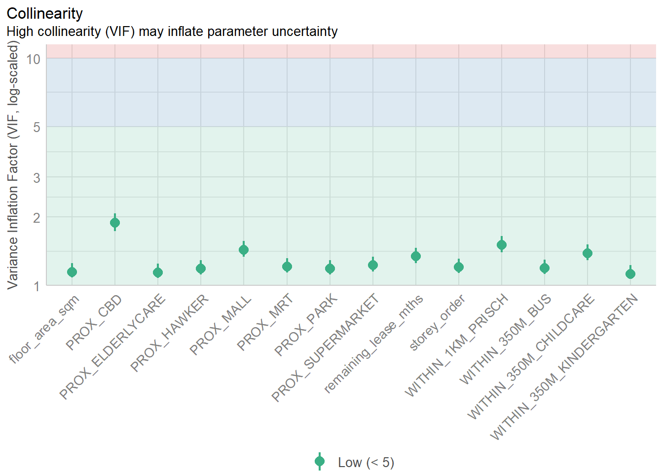
7. Predictive Modelling with gwr
7.1 Computing adaptive bandwidth
bw_adaptive <- bw.gwr(resale_price ~ floor_area_sqm +
                  storey_order + remaining_lease_mths +
                  PROX_CBD + PROX_ELDERLYCARE + PROX_HAWKER +
                  PROX_MRT + PROX_PARK + PROX_MALL +
                  PROX_SUPERMARKET + WITHIN_350M_KINDERGARTEN +
                  WITHIN_350M_CHILDCARE + WITHIN_350M_BUS +
                  WITHIN_1KM_PRISCH,
                  data=train_data,
                  approach="CV",
                  kernel="gaussian",
                  adaptive=TRUE,
                  longlat=FALSE)
Adaptive bandwidth: 625 CV score: 3.459032e+12
Adaptive bandwidth: 394 CV score: 3.231786e+12
Adaptive bandwidth: 250 CV score: 2.914736e+12
Adaptive bandwidth: 162 CV score: 2.610897e+12
Adaptive bandwidth: 107 CV score: 2.240188e+12
Adaptive bandwidth: 73 CV score: 1.971641e+12
Adaptive bandwidth: 52 CV score: 1.797271e+12
Adaptive bandwidth: 39 CV score: 1.659472e+12
Adaptive bandwidth: 31 CV score: 1.573963e+12
Adaptive bandwidth: 26 CV score: 1.550147e+12
Adaptive bandwidth: 23 CV score: 1.542544e+12
Adaptive bandwidth: 21 CV score: 1.518885e+12
Adaptive bandwidth: 19 CV score: 1.515965e+12
Adaptive bandwidth: 19 CV score: 1.515965e+12 bw_adaptive[1] 197.2 Model calibration
gwr_adaptive <- gwr.basic(formula = resale_price ~
                            floor_area_sqm + storey_order +
                            remaining_lease_mths + PROX_CBD +
                            PROX_ELDERLYCARE + PROX_HAWKER +
                            PROX_MRT + PROX_PARK + PROX_MALL +
                            PROX_SUPERMARKET + WITHIN_350M_KINDERGARTEN +
                            WITHIN_350M_CHILDCARE + WITHIN_350M_BUS +
                            WITHIN_1KM_PRISCH,
                          data=train_data,
                          bw=bw_adaptive,
                          kernel = 'gaussian',
                          adaptive=TRUE,
                          longlat = FALSE)
gwr_adaptive ***********************************************************************
* Package GWmodel *
***********************************************************************
Program starts at: 2024-11-01 00:47:17.198423
Call:
gwr.basic(formula = resale_price ~ floor_area_sqm + storey_order +
remaining_lease_mths + PROX_CBD + PROX_ELDERLYCARE + PROX_HAWKER +
PROX_MRT + PROX_PARK + PROX_MALL + PROX_SUPERMARKET + WITHIN_350M_KINDERGARTEN +
WITHIN_350M_CHILDCARE + WITHIN_350M_BUS + WITHIN_1KM_PRISCH,
data = train_data, bw = bw_adaptive, kernel = "gaussian",
adaptive = TRUE, longlat = FALSE)
Dependent (y) variable: resale_price
Independent variables: floor_area_sqm storey_order remaining_lease_mths PROX_CBD PROX_ELDERLYCARE PROX_HAWKER PROX_MRT PROX_PARK PROX_MALL PROX_SUPERMARKET WITHIN_350M_KINDERGARTEN WITHIN_350M_CHILDCARE WITHIN_350M_BUS WITHIN_1KM_PRISCH
Number of data points: 1000
***********************************************************************
* Results of Global Regression *
***********************************************************************
Call:
lm(formula = formula, data = data)
Residuals:
Min 1Q Median 3Q Max
-167624 -37265 -415 34811 224601
Coefficients:
Estimate Std. Error t value Pr(>|t|)
(Intercept) 115703.7 34303.4 3.373 0.000773 ***
floor_area_sqm 2778.6 292.3 9.507 < 2e-16 ***
storey_order 12698.2 1071.0 11.857 < 2e-16 ***
remaining_lease_mths 350.2 14.6 23.997 < 2e-16 ***
PROX_CBD -16225.6 630.1 -25.751 < 2e-16 ***
PROX_ELDERLYCARE -11330.9 3220.8 -3.518 0.000455 ***
PROX_HAWKER -19964.1 4021.1 -4.965 8.10e-07 ***
PROX_MRT -39652.5 5412.3 -7.326 4.92e-13 ***
PROX_PARK -15878.3 4609.2 -3.445 0.000595 ***
PROX_MALL -15910.9 6438.1 -2.471 0.013628 *
PROX_SUPERMARKET -18928.5 13305.0 -1.423 0.155150
WITHIN_350M_KINDERGARTEN 9309.7 2024.3 4.599 4.80e-06 ***
WITHIN_350M_CHILDCARE -1619.5 1181.0 -1.371 0.170572
WITHIN_350M_BUS -447.7 738.7 -0.606 0.544624
WITHIN_1KM_PRISCH -10698.0 1543.5 -6.931 7.55e-12 ***
---Significance stars
Signif. codes: 0 '***' 0.001 '**' 0.01 '*' 0.05 '.' 0.1 ' ' 1
Residual standard error: 61270 on 985 degrees of freedom
Multiple R-squared: 0.7424
Adjusted R-squared: 0.7387
F-statistic: 202.7 on 14 and 985 DF, p-value: < 2.2e-16
***Extra Diagnostic information
Residual sum of squares: 3.698259e+12
Sigma(hat): 60874.22
AIC: 24901.01
AICc: 24901.56
BIC: 24090.05
***********************************************************************
* Results of Geographically Weighted Regression *
***********************************************************************
*********************Model calibration information*********************
Kernel function: gaussian
Adaptive bandwidth: 19 (number of nearest neighbours)
Regression points: the same locations as observations are used.
Distance metric: Euclidean distance metric is used.
****************Summary of GWR coefficient estimates:******************
Min. 1st Qu. Median 3rd Qu.
Intercept -1850662.06 -213226.88 18750.18 257759.31
floor_area_sqm -4400.58 1227.91 2020.59 3305.91
storey_order 3226.46 8118.79 10349.25 13840.12
remaining_lease_mths -567.87 343.26 422.16 502.70
PROX_CBD -107227.77 -23329.41 -10632.77 -983.94
PROX_ELDERLYCARE -262405.86 -25815.67 -5892.75 18397.75
PROX_HAWKER -217237.20 -36313.19 -9931.90 21441.49
PROX_MRT -305069.89 -92410.01 -57000.64 -20410.27
PROX_PARK -256758.99 -33742.57 -16756.73 8462.87
PROX_MALL -274223.06 -35730.88 6953.21 49221.11
PROX_SUPERMARKET -176209.93 -43225.75 -7954.90 30114.02
WITHIN_350M_KINDERGARTEN -43387.03 -9117.13 -2525.06 5559.95
WITHIN_350M_CHILDCARE -15152.19 -2203.26 1242.91 3469.04
WITHIN_350M_BUS -10848.37 -1806.81 523.89 2318.23
WITHIN_1KM_PRISCH -50593.97 -4155.12 348.43 4951.49
Max.
Intercept 1668279.80
floor_area_sqm 7834.73
storey_order 26827.97
remaining_lease_mths 792.01
PROX_CBD 130929.41
PROX_ELDERLYCARE 178770.13
PROX_HAWKER 146976.62
PROX_MRT 126271.80
PROX_PARK 90469.23
PROX_MALL 342520.92
PROX_SUPERMARKET 189007.16
WITHIN_350M_KINDERGARTEN 40812.13
WITHIN_350M_CHILDCARE 15729.60
WITHIN_350M_BUS 11766.10
WITHIN_1KM_PRISCH 32922.16
************************Diagnostic information*************************
Number of data points: 1000
Effective number of parameters (2trace(S) - trace(S'S)): 419.14
Effective degrees of freedom (n-2trace(S) + trace(S'S)): 580.86
AICc (GWR book, Fotheringham, et al. 2002, p. 61, eq 2.33): 24103.65
AIC (GWR book, Fotheringham, et al. 2002,GWR p. 96, eq. 4.22): 23393.52
BIC (GWR book, Fotheringham, et al. 2002,GWR p. 61, eq. 2.34): 24424.31
Residual sum of squares: 5.99674e+11
R-square value: 0.9582264
Adjusted R-square value: 0.9280312
***********************************************************************
Program stops at: 2024-11-01 00:47:17.992583 8. Predictive Modelling with MLR
8.1 Predicting with test data
Test data bw
gwr_bw_test_adaptive <- bw.gwr(resale_price ~ floor_area_sqm +
                  storey_order + remaining_lease_mths +
                  PROX_CBD + PROX_ELDERLYCARE + PROX_HAWKER +
                  PROX_MRT + PROX_PARK + PROX_MALL +
                  PROX_SUPERMARKET + WITHIN_350M_KINDERGARTEN +
                  WITHIN_350M_CHILDCARE + WITHIN_350M_BUS +
                  WITHIN_1KM_PRISCH,
                  data=test_data,
                  approach="CV",
                  kernel="gaussian",
                  adaptive=TRUE,
                  longlat=FALSE)
Adaptive bandwidth: 316 CV score: 1.752181e+12
Adaptive bandwidth: 203 CV score: 1.635856e+12
Adaptive bandwidth: 132 CV score: 1.452381e+12
Adaptive bandwidth: 89 CV score: 1.292305e+12
Adaptive bandwidth: 61 CV score: 1.115867e+12
Adaptive bandwidth: 45 CV score: 1.007764e+12
Adaptive bandwidth: 34 CV score: 886240690082
Adaptive bandwidth: 28 CV score: 859792519354
Adaptive bandwidth: 23 CV score: 856247388819
Adaptive bandwidth: 21 CV score: 846203688028
Adaptive bandwidth: 19 CV score: 837013751208
Adaptive bandwidth: 18 CV score: 8.32968e+11
Adaptive bandwidth: 17 CV score: 834218488856
Adaptive bandwidth: 18 CV score: 8.32968e+11 Predicting
gwr_pred <- gwr.predict(formula = resale_price ~
                          floor_area_sqm + storey_order +
                          remaining_lease_mths + PROX_CBD +
                          PROX_ELDERLYCARE + PROX_HAWKER +
                          PROX_MRT + PROX_PARK + PROX_MALL +
                          PROX_SUPERMARKET + WITHIN_350M_KINDERGARTEN +
                          WITHIN_350M_CHILDCARE + WITHIN_350M_BUS +
                          WITHIN_1KM_PRISCH,
                        data=train_data,
                        predictdata = test_data,
                        bw=bw_adaptive,
                        kernel = 'gaussian',
                        adaptive=TRUE,
                        longlat = FALSE)
9. Predictive Modelling: RF method
9.1 Data Preparation
Firstly, code chunk below is used to extract the coordinates of training and test data sets
coords <- st_coordinates(HDB_sample)
coords_train <- st_coordinates(train_data)
coords_test <- st_coordinates(test_data)
Next, code chunk below is used to drop the geometry column of both training and test data sets.
train_data_nogeom <- train_data %>%
  st_drop_geometry()
9.2 Calibrating RF model
set.seed(1234)
rf <- ranger(resale_price ~ floor_area_sqm + storey_order +
               remaining_lease_mths + PROX_CBD + PROX_ELDERLYCARE +
               PROX_HAWKER + PROX_MRT + PROX_PARK + PROX_MALL +
               PROX_SUPERMARKET + WITHIN_350M_KINDERGARTEN +
               WITHIN_350M_CHILDCARE + WITHIN_350M_BUS +
               WITHIN_1KM_PRISCH,
             data=train_data_nogeom)
9.3 Model output
rfRanger result
Call:
ranger(resale_price ~ floor_area_sqm + storey_order + remaining_lease_mths + PROX_CBD + PROX_ELDERLYCARE + PROX_HAWKER + PROX_MRT + PROX_PARK + PROX_MALL + PROX_SUPERMARKET + WITHIN_350M_KINDERGARTEN + WITHIN_350M_CHILDCARE + WITHIN_350M_BUS + WITHIN_1KM_PRISCH, data = train_data_nogeom)
Type: Regression
Number of trees: 500
Sample size: 1000
Number of independent variables: 14
Mtry: 3
Target node size: 5
Variable importance mode: none
Splitrule: variance
OOB prediction error (MSE): 2289284270
R squared (OOB): 0.8406868 10. Predictive Modelling: SpatialML method
Calibrating with grf
set.seed(1234)
gwRF_adaptive <- grf(formula = resale_price ~ floor_area_sqm +
                       storey_order + remaining_lease_mths +
                       PROX_CBD + PROX_ELDERLYCARE + PROX_HAWKER +
                       PROX_MRT + PROX_PARK + PROX_MALL +
                       PROX_SUPERMARKET + WITHIN_350M_KINDERGARTEN +
                       WITHIN_350M_CHILDCARE + WITHIN_350M_BUS +
                       WITHIN_1KM_PRISCH,
                     dframe=train_data_nogeom,
                     bw=55,
                     kernel="adaptive",
                     coords=coords_train)
Number of Observations: 1000Number of Independent Variables: 14Kernel: Adaptive
Neightbours: 55
--------------- Global ML Model Summary ---------------Ranger result
Call:
ranger(resale_price ~ floor_area_sqm + storey_order + remaining_lease_mths + PROX_CBD + PROX_ELDERLYCARE + PROX_HAWKER + PROX_MRT + PROX_PARK + PROX_MALL + PROX_SUPERMARKET + WITHIN_350M_KINDERGARTEN + WITHIN_350M_CHILDCARE + WITHIN_350M_BUS + WITHIN_1KM_PRISCH, data = train_data_nogeom, num.trees = 500, mtry = 4, importance = "impurity", num.threads = NULL)
Type: Regression
Number of trees: 500
Sample size: 1000
Number of independent variables: 14
Mtry: 4
Target node size: 5
Variable importance mode: impurity
Splitrule: variance
OOB prediction error (MSE): 2056587170
R squared (OOB): 0.8568804
Importance: floor_area_sqm storey_order remaining_lease_mths
6.932661e+11 1.471090e+12 2.512971e+12
PROX_CBD PROX_ELDERLYCARE PROX_HAWKER
4.695331e+12 5.430899e+11 6.061641e+11
PROX_MRT PROX_PARK PROX_MALL
8.355142e+11 5.612980e+11 4.449032e+11
PROX_SUPERMARKET WITHIN_350M_KINDERGARTEN WITHIN_350M_CHILDCARE
3.698543e+11 1.287529e+11 2.290324e+11
WITHIN_350M_BUS WITHIN_1KM_PRISCH
2.310307e+11 7.644464e+11
Mean Square Error (Not OOB): 398120142.153R-squared (Not OOB) %: 97.227AIC (Not OOB): 19832.264AICc (Not OOB): 19832.752
--------------- Local Model Summary ---------------
Residuals OOB: Min. 1st Qu. Median Mean 3rd Qu. Max.
-221080.0 -21530.3 -895.4 -271.1 20305.0 296404.4
Residuals Predicted (Not OOB): Min. 1st Qu. Median Mean 3rd Qu. Max.
-38672.86 -3227.99 -178.43 -71.12 2831.66 42872.18
Local Variable Importance: Min Max Mean StD
floor_area_sqm 696919686 192865321765 24393255920 32201130831
storey_order 517785315 319895669535 27780386721 50723636275
remaining_lease_mths 2957069739 610102523068 100407363399 137038263288
PROX_CBD 962467743 343722236312 30938242726 48859511192
PROX_ELDERLYCARE 1897793617 150381230352 23249130891 25384606673
PROX_HAWKER 1035238085 214011373785 20753714949 24523766193
PROX_MRT 1130621303 267464693079 28928314326 46397690636
PROX_PARK 1137628579 179606297600 19965989625 21334314778
PROX_MALL 1278390826 271590767488 27256268534 40402723719
PROX_SUPERMARKET 991735075 176833138872 18996601028 27059219290
WITHIN_350M_KINDERGARTEN 173811210 49153266122 5742647253 7358559963
WITHIN_350M_CHILDCARE 445891832 182607185549 18494577567 33745415431
WITHIN_350M_BUS 590779439 142390607080 9066032058 11317330875
WITHIN_1KM_PRISCH 220777233 60582254997 6408000068 7434712348
Mean squared error (OOB): 2102566645.863R-squared (OOB) %: 85.353AIC (OOB): 21496.425AICc (OOB): 21496.912Mean squared error Predicted (Not OOB): 51423033.017R-squared Predicted (Not OOB) %: 99.642AIC Predicted (Not OOB): 17785.597AICc Predicted (Not OOB): 17786.085
Calculation time (in seconds): 40.944811. Predicting by using the test data
11.1 Preparing the test data
test_data_nogeom <- cbind(
  test_data, coords_test) %>%
  st_drop_geometry()
11.2 Predicting with the test data
In the code chunk below, predict.grf() of spatialML for predicting re-sale prices in the test data set (i.e. test_data_nogeom)
gwRF_pred <- predict.grf(gwRF_adaptive,
                           test_data_nogeom,
                           x.var.name="X",
                           y.var.name="Y",
                           local.w=1,
global.w=0)str(gwRF_pred) num [1:500] 424497 495806 376473 372622 377314 ...11.3 Creating DF
Next, the code chunk below is used to convert the output from predict.grf() into a data.frame.
GRF_pred_df <- as.data.frame(gwRF_pred)nrow(GRF_pred_df)[1] 500Then, cbind() is used to append fields in GRF_pred_df data.frame onto test_data.
test_data_pred <- cbind(test_data,
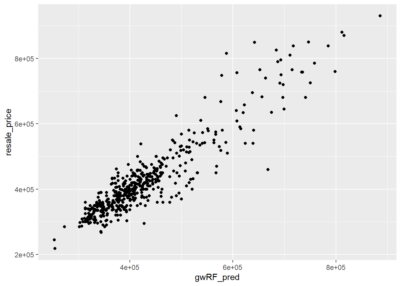
GRF_pred_df)12. Visualising the predicted values
ggplot(data = test_data_pred,
       aes(x = gwRF_pred,
           y = resale_price)) +
  geom_point()